Original solutions to all nine questions and all thirteen terminal parts. Source: released Mathematics examination papers, archive
FOI 20210708 1 Data.zip, examination of 23 June 2005.Let be the minimal polynomial. If with , then , so . Conversely, if , write . If were invertible, the identity would imply , contradicting minimality of the degree. Thus has a nonzero kernel of a linear map, and is an eigenvalue. This proves the eigenvalue criterion using the minimal polynomial for roots in the field under consideration.
For the given matrix, direct expansion givesPut . Direct multiplication givesBy the Cayley-Hamilton theorem, divides ; the nonzero square rules out every smaller power. Therefore . Its sole eigenvalue is , but the size of the nilpotent part makes the minimum polynomial cubic rather than linear.
For affine polynomials and , direct integration gives . This is bilinear and symmetric, and for every nonzero . Thus it is an inner product.
The adjoint of differentiation on affine polynomials is determined by . Since , the left side is . Writing , the right side is . Equality for every forces , , henceThis is not simply negative differentiation: there are no endpoint conditions here that would remove the boundary term in an integration by parts argument.
An ideal is an additive subgroup of a ring closed under multiplication by arbitrary ring elements; in a potentially noncommutative ring, a two-sided ideal must absorb multiplication on both sides. For a ring homomorphism , its kernel of a ring homomorphism contains zero, is closed under subtraction, and satisfies and . Thus is an ideal.
Define by . It is well-defined because two representatives differ by an element of , preserves addition and multiplication, is surjective by hypothesis, and is injective because its zero class is precisely . Therefore , the first isomorphism theorem for rings.
Apply this to the evaluation homomorphism , . Constants prove surjectivity, and division by shows that its kernel of a ring homomorphism is . Hence .
For a smooth curve and continuous on its image, the contour integral is defined byThe derivative carries the direction and speed of traversal; the complex-valued real-parameter integral is defined by integrating its real and imaginary parts.
The chain rule gives . The fundamental theorem of calculus therefore yieldsbecause the closed curve has equal endpoints. The existence of a single-valued holomorphic antiderivative on the whole neighborhood is the decisive hypothesis.
Take the unit circle , , in the punctured complex plane. Direct parameter integration givesA global holomorphic antiderivative would make this integral zero by the previous part. Thus there is no such antiderivative on the punctured plane. Local primitives can exist without combining into one single-valued function on this domain.
If a holomorphic function on the punctured complex plane satisfied , the chain rule would give , hence . This contradicts the previous part. Therefore there is no global holomorphic logarithm on the punctured plane. A branch of the complex logarithm requires a suitable smaller domain.
A pole of order at means that near , where is holomorphic and . Equivalently its Laurent series has a finite principal part with leading nonzero term . The residue is the coefficient . For a simple pole, , this coefficient is , soFor , the zeros of the denominator are exactly , : this follows from . Each is simple, because . ThereforeThere are no other finite singularities. If infinity is included, it is an accumulation point of these poles, so it is not an isolated singularity to which the usual removable/pole/essential classification could be applied.
A Möbius transformation has the form with , extended to the Riemann sphere by its limiting values at its pole and at infinity. If , it sends to infinity and infinity to ; if , infinity maps to infinity.
Represent by the invertible matrix , with nonzero scalar multiples representing the same map. Substitution shows that composition corresponds to matrix multiplication. The product determinant is the product of two nonzero determinants, so the composition is again a Möbius transformation. Solving giveswith the same extended-value convention. This inverse proves that is a bijection of the extended complex plane.
Use the Cayley transformFor , its denominator is nonzero, and direct subtraction gives . Thus the image lies in the open unit disk. Conversely, for the inverse is , with . Hence it maps the upper half-plane bijectively onto the disk.
Since the exponential factor is positive, equilibria must have and . Thus . At either point the Jacobian matrix is . At its eigenvalues are , so this is a saddle point. At they are : the linearization has a centre equilibrium.
The requested first-order approximation follows by putting , : and . The linearized system conserves , giving the approximate ellipsesHowever, the printed nonlinear system has a weak repelling focus at , rather than a centre. A centre in the linearization need not be a nonlinear centre. Here that distinction can be proved explicitly, without relying on the numerical drift in the figure.
Put , , and . The weak focus of an exponential polynomial planar system has the local positive functionExpanding the vector field through cubic order and differentiating givesThe cubic correction cancels the cubic terms in the derivative of , and the quartic correction leaves the positive radial term . Since is positive and the angular velocity stays near , small nonzero trajectories spiral outward. Equivalently the reversed system has a strict local Lyapunov function and an asymptotically stable equilibrium. In particular, a periodic orbit sufficiently near the equilibrium is impossible, because would have to increase strictly and return to its starting value. This proves the failure of the printed centre assertion while retaining its correct linearized ellipse calculation.
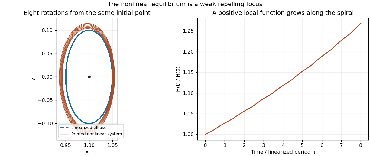
The linearized ellipses hide the nonlinear outward spiral
. Original fourth-order Runge-Kutta integration of the printed vector field, compared with its linearization from the same initial point. The local polynomial calculation, rather than the plot, proves the weak instability. Details.
The characteristic equations for a first-order quasilinear equation are , , , with characteristic parameter . Through the prescribed point they giveFor a nonzero projected initial point, the characteristic projections are rays from the origin, not trajectories crossing through the origin to the opposite ray. If , a classical solution graph requires , because the original equation reduces there to .
Parameterize the initial line by . Along its characteristic, , and . ThereforeDifferentiation verifies the equation, and substitution of verifies the initial data. Characteristic reachability for radial transport shows why the domain is this positive half-plane: each point there lies on precisely one characteristic from the data line. Rays in never meet that line, so their values are not determined by these data. Allowing a negative scaling factor would incorrectly join two different characteristic rays through a degenerate origin.
Integrating , or taking the imaginary part of , givesThe Laplace transform convolution theorem states whenever the transforms and convolution are defined. Applying it to the Volterra integral equation gives , soSince , a second application of the convolution theorem yields the sine-kernel Volterra resolventThe transform argument assumes suitable growth for the transforms to exist. The resulting causal resolvent formula also applies to locally integrable forcing on finite intervals, as can be checked by substitution and exchanging integrals over a finite triangle.
Articles by others on the same topic
There are currently no matching articles.