Past exam of the algebra, analysis and differential equations II course of the University of Oxford / 2011 (AC2, XMAT 4302, XMST 4302)

Source: Mathematics release, supplied bundle Part A 2007 11-1.pdf, pages 265–272. The eight-page paper is dated 28 June 2011 and covers Mathematics and Mathematics & Statistics Part A.

The department's answer-release policy excludes ordinary odd years. Bounded exact-paper searches found no matching full or selected answer advertisement, so no parts are skipped. All printed parts and their surrounding unnumbered requests are answered below.

Choose a basis and let $A$ represent $T$. Define the characteristic polynomial byUnder a change of basis with invertible change matrix $S$, the new matrix is $S^{-1}AS$. HenceThus the polynomial is independent of the chosen coordinates. It is monic of degree $\dim V$.

To prove the sum is direct, suppose ${\sum }_{j=1}^r{v}_j=0$ with $v_j\in V_{{\lambda }_j}$. Fix $i$ and apply the polynomial in the linear operatorEvery $v_j$ with $j\ne i$ is killed by one factor. On $v_i$, each factor is multiplication by ${\lambda }_i-{\lambda }_j$, givingThe scalar coefficient is nonzero because the eigenvalues are distinct. Thus $v_i=0$ for every $i$, provingIn particular, choosing a basis in each eigenspace yields a linearly independent combined list.

If ${\chi }_T(\lambda )=0$, then $\det (\lambda I-A)=0$, so $\lambda I-A$ is singular. By the rank-nullity theorem it has a nonzero kernel vector $v$. ThusThis is exactly the definition of an eigenvalue. Here $\lambda$ lies in the scalar field: for the stated real vector space it is real. A nonreal root instead gives an eigenvalue of the complexified operator, by the same argument over $\mathbb{C}$.

Expanding the determinant along the second column givesIf $b\notin \{-3,2\}$, there are three distinct real eigenvalues. Part (b)(ii) gives a nonzero eigenvector for each, and part (b)(i) makes them independent. They form a basis, so the matrix is diagonalisable.

When $b=-3$,has rank one for every $a$: the third row is nonzero, and the second row is $a/5$ times the third. Therefore the eigenspace for $-3$ has dimension two. The eigenvalue $2$ provides at least one further independent eigenvector by part (b), so again there is an eigenbasis.

When $b=2$,Its rank is one if $a=0$ and two otherwise. Thus the eigenspace for $2$ has dimension two exactly when $a=0$. For $a\ne 0$ it has dimension one, while the eigenspace for $-3$ also has dimension one, since $X+3I$ then has rank two. There are no other eigenvalues by the characteristic polynomial. A diagonal matrix in an eigenbasis would need three independent eigenvectors, whereas these two eigenspaces supply only two; diagonalisation is impossible. Conversely, at $a=0$ their dimensions add to three and part (b) makes their sum direct. ThereforeThe argument uses only the determinant, rank-nullity, the established direct-sum result, and the definition of diagonalisation.

Use the convention that the inner product is linear in its first argument, as required by the displayed representation of a linear functional. Choose an orthonormal basis $e_1,\dots ,e_n$, for instance by Gram-Schmidt orthogonalization. DefineFor $u={\sum }_j{u}_j{e}_j$, conjugate linearity in the second argument givesThusThe representation is unique as well: if two vectors represent the same functional, their difference is orthogonal to every vector and therefore to itself, so it is zero.

The adjoint operator is characterized byFor each fixed $v$, the map $u\mapsto ⟨Tu,v⟩$ is a linear functional. Part (i) gives a representing vector, which we define to be $T^{\ast }v$. Hence such a map exists on every vector of $V$. Part (b) proves that this constructed map is linear.

For scalars $\alpha ,\beta$ and vectors $v,w,u$, use the adjoint identity and conjugate linearity in the second argument:The difference of the two second-argument vectors is orthogonal to every $u$. Choosing $u$ to be that difference shows its squared norm is zero. ThereforeThe two conjugations are why the adjoint is a linear map, despite the conjugate-linear dependence of the representing functional on its second argument.

The finite-dimensional spectral theorem says that a self-adjoint operator on a complex inner-product space has an orthonormal basis of eigenvectors and all its eigenvalues are real. Equivalently, its matrix is unitarily diagonalisable with real diagonal entries.

For $a\in \mathbb{R}$, the matrix is equal to its conjugate transpose:Thus it represents a self-adjoint operator for the standard inner product on ${\mathbb{C}}^3$. The theorem applies directly, proving

Set $N=M_i-I$. Direct multiplication giveswith $N\ne 0$. If $M_i$ were diagonalisable, then subtracting the identity in the same basis would diagonalise $N$. A diagonal matrix whose cube is zero has every diagonal entry zero and is itself zero. Similarity would then imply $N=0$, a contradiction. HenceThis proves failure directly; merely observing that it is not self-adjoint would not suffice, because non-self-adjoint matrices can still be diagonalisable.

An ideal $I$ of a commutative ring is an additive subgroup such that $rx\in I$ for every $r\in R$ and $x\in I$. A prime ideal is a proper ideal $A\ne R$ such that $xy\in A$ implies $x\in A$ or $y\in A$.

If $(x+A)(y+A)=0+A$ in the quotient ring, then $xy\in A$. Primality implies $x+A=0+A$ or $y+A=0+A$. Therefore there are no two nonzero cosets whose product is zero:Properness also ensures its identity coset is not zero, so this quotient is an integral domain.

The set $\sqrt{I}$ contains zero. If $x^m\in I$, then $(-x{)}^m=(-1{)}^m{x}^m\in I$, giving closure under additive inverses; also $(rx{)}^m=r^m{x}^m\in I$ for every $r\in R$.

To prove closure under addition, let $x^m,y^n\in I$. Expand $(x+y{)}^{m+n-1}$ by the binomial theorem. In every monomial $x^j{y}^{m+n-1-j}$, either $j\ge m$ or $m+n-1-j\ge n$. Thus each term contains a factor $x^m$ or $y^n$ and belongs to $I$. Hence $(x+y{)}^{m+n-1}\in I$, so $x+y\in \sqrt{I}$. The additive subgroup and absorption properties are proved, givingThis ideal is the radical of an ideal. The finite exponent for a sum uses commutativity of the ring.

A coset is a nilpotent element of the quotient exactly when some positive power is zero:If $J=\sqrt{J}$, this forces every nilpotent coset to equal zero. Conversely, if there is no nonzero nilpotent coset, every $x\in \sqrt{J}$ has $x+J=0$, hence $x\in J$. Since $J\subseteq \sqrt{J}$ always, equality follows. ThereforeIn standard terms, an ideal is radical exactly when its quotient is a reduced ring.

Certainly $A\subseteq \sqrt{A}$, by taking exponent one. If $x\in \sqrt{A}$, choose $n\ge 1$ with $x^n\in A$. Primality applied to $x\cdot x^{n-1}$ gives $x\in A$ or $x^{n-1}\in A$. In the latter case repeat; induction reduces to $x\in A$. Thus $\sqrt{A}\subseteq A$ as well, provingEvery prime ideal is therefore a radical ideal.

For the preliminary definition, put $S_N(z)={\sum }_{k=1}^N{f}_k(z)$. The series converges uniformly to $f$ on $U$ when, for every $ϵ>0$, some $N_0$ satisfies $|S_N(z)-f(z)|<ϵ$ for all $z\in U$ and all $N\ge N_0$. Equivalently, ${\sup }_{z\in U}|S_N(z)-f(z)|\to 0$.

Let $L(\gamma )$ be the finite length of the piecewise-smooth path. Finite linearity of the contour integral and the integral bound giveThe uniform limit is continuous by the stated allowed result, so its integral is defined. Consequently

Cauchy's integral theorem states that if a function is holomorphic on a simply connected open set, its integral around every closed piecewise-smooth path in that set is zero. A local form sufficient here is: if a function is holomorphic on an open set containing a triangle together with its interior, thenFor a general domain with holes, an arbitrary closed path need not have zero integral; the triangle or simple-connectedness hypothesis supplies the required interior.

Morera's theorem states that if $f$ is continuous on an open set $U$ and its integral around every triangle whose interior and boundary lie in $U$ is zero, then $f$ is holomorphic on $U$.

For a proof, choose a disk $B\subseteq U$ and a base point $z_0\in B$. Define $F(z)={\int }_{[z_0,z]}f(\zeta )d\zeta$ along the straight segment. Convexity keeps every triangle with vertices $z_0,z,z+h$ inside $B$. Its zero boundary integral impliesBy continuity, the last integral tends to $f(z)$ as $h\to 0$, so $F^{\prime }(z)=f(z)$. Thus $F$ is holomorphic on $B$. The allowed result that the derivative of a holomorphic function is holomorphic now gives that $f=F^{\prime }$ is holomorphic there. Such disks cover $U$, proving

For each triangle compactly contained in $U$, part (i) permits the interchange of the series and its boundary integral. Cauchy's integral theorem makes every term zero. The uniform limit is continuous, so Morera's theorem yields that $f$ is holomorphic on $U$.

For the final application, each function $(z-k{)}^{-2}$ is holomorphic away from its pole. Fix a positive integer $n$. For $z\in U_n$ and $k>2n$,The numerical series ${\sum }_{k>2n}4/k^2$ converges, so the Weierstrass M-test gives uniform convergence of the tail on $U_n$. Adding the finitely many initial terms preserves uniform convergence. Those initial terms need not be bounded near their excluded poles; only the tail needs the uniform bound. By the first conclusion, the full sum is holomorphic on each $U_n$. Their union is $\mathbb{C}\setminus \mathbb{N}$, hence

The residue at $a$ is the coefficient $c_{-1}$ of $(z-a{)}^{-1}$ in the Laurent series. A simple pole means $f(z)=c_{-1}/(z-a)+h(z)$ near $a$, with $c_{-1}\ne 0$ and $h$ holomorphic across $a$.

For the specified positively oriented arc, direct parametrization gives ${\int }_{{\gamma }_{ϵ}}(z-a{)}^{-1}dz=i(\beta -\alpha )$. The remaining integral is bounded by $ϵ(\beta -\alpha )\sup |h|$, which tends to zero because $h$ is bounded near $a$. ThereforeThe simple-pole hypothesis matters. For $f(z)=(z-a{)}^{-2}$, with $\alpha =0$, $\beta =\pi$, the residue is zero butFor the particular function, expanding the exponential givesThus $\boxed{\mathrm{res}(f;0)=1/2}$, and the pole is simple. On the large upper semicircle, $|e^{iz}|\le 1$, givingClose the real-axis path from $-R$ to $-ϵ$ and $ϵ$ to $R$ by this upper arc and a clockwise upper indentation at zero. The function is holomorphic in the indented region, so the sum of all four integrals is zero. The clockwise indentation tends to $-i\pi /2$. For real $x$,The real part is odd and cancels on the symmetric real pieces; the imaginary part is even. Its integral converges since $(x-\sin x)/x^3\to 1/6$ at zero and is $O(x^{-2})$ at infinity. Letting $ϵ\to 0$ and $R\to \infty$ therefore yields $2iI-i\pi /2=0$, where $I$ is the requested real integral. Hence

A conformal map preserves angles between intersecting regular curves, including their orientation. If $f$ is holomorphic with $f^{\prime }(a)\ne 0$, the image tangent vectors are $f^{\prime }(a)$ times the original tangent vectors. Multiplication by this nonzero complex number gives a common positive scaling and rotation, so their oriented angle is unchanged. This proves conformality throughout the stated domain.

At a zero derivative this can fail: $f(z)=z^2$ at zero sends rays of arguments $0$ and $\pi /4$ to rays of arguments $0$ and $\pi /2$. The angle is doubled, so this holomorphic function is not conformal there.

For the disk map $C(z)=i(1+z)/(1-z)$, computeIts inverse is $z=(w-i)/(w+i)$; for $\mathrm{Im}w>0$, the inequality $|w-i|<|w+i|$ puts this inverse in the unit disk. Both rational maps are holomorphic on their respective domains. ThusFor the final region, writing $z=x+iy$ gives $|e^z|=e^x\in (0,1)$ and $\arg (e^z)=y\in (0,\pi )$. Hence its exponential image is exactly the upper half of the unit disk,The exponential is injective on this strip, since two equal exponential values differ by $2\pi i$ times an integer while the imaginary parts here differ by less than $\pi$. Its derivative never vanishes and its inverse on $V$ is the logarithm with argument in $(0,\pi )$.

Now $L(w)=(1+w)/(1-w)$ maps $V$ conformally onto the first quadrant. Indeedand the inverse $(s-1)/(s+1)$ has modulus below one and positive imaginary part for every first-quadrant $s$. Squaring maps that quadrant bijectively onto $\mathbb{H}$, with nonzero derivative. Therefore a required composition isEvery component is a conformal bijection between the stated domains, so the composition is one as well.

First prove the general uniqueness claim. The bound $Mh\le k$ prevents a solution from leaving the dependent-variable interval before $|x-a|=h$: up to any first exit, $|y(x)-b|\le M|x-a|\le k$. Let $y_1,y_2$ be two solutions with the same initial value. Their integral equations and the Lipschitz condition give, for $x\ge a$,Since their difference is bounded by $2k$, repeated substitution into this inequality proves, for every integer $n\ge 0$,The same argument with reversed limits works for $x\le a$. Letting $n\to \infty$ forces the difference to zero on the whole interval. This proves at most one solution without assuming that $Ah<1$.

For case (i), choose a rectangle around $(0,1)$ that stays in $y>0$. There $f_y=(2/3)x{y}^{-1/3}$ is bounded, giving a uniform Lipschitz constant by the mean value theorem. For example $h=k=1/2$ works: $M\le \frac{1}{2}(3/2{)}^{2/3}$ and $Mh<1/2$. Separate variables using $u=y^{1/3}$, obtaining $3u^{\prime }=x$. The initial condition gives $u=1+x^2/6$, henceIt remains positive for all real $x$, so the same local uniqueness argument continues along this solution.

No rectangle of positive width around $(0,0)$ has a uniform Lipschitz constant in $y$. For any nonzero $x$ in such a rectangle,The vanishing factor $x$ at the single initial point does not control neighbouring $x$-values. The failure of the hypothesis is accompanied by actual nonuniqueness: bothsatisfy the equation and have value zero at $x=0$. Direct differentiation gives $y_2^{\prime }=x^5/36=x(y_2{)}^{2/3}$, including the zero point by continuity.

The same quotient $|x||y{|}^{-1/3}$ is unbounded near $(1,0)$, so the uniform Lipschitz hypothesis again fails. Two explicit solutions through the initial point areFor the second, put $u=(x^2-1)/6$. Then $y_2^{\prime }=3u^2(x/3)=x{u}^2=x(y_2{)}^{2/3}$, and $y_2(1)=0$. The real power here means the square of the real cube root, so the identity also holds when $y_2$ is negative. Both functions are differentiable through their zeros. Thus uniqueness fails in this case as well.

For a nonzero second-order principal part, the discriminant is $Q^2-PR$: positive gives a hyperbolic partial differential equation, negative an elliptic partial differential equation, and zero the parabolic type when the principal part has rank one. If all three coefficients vanish, the equation is instead degenerate to lower order.

Here $P=x$, $2Q=x^2$, $R=0$, so $Q^2-PR=x^4/4>0$ for $x>0$. The characteristic equation isThus chooseTheir Jacobian determinant with respect to $(x,y)$ is $x\ne 0$, so they are valid coordinates on the specified half-plane. The level sets are horizontal lines and the right-hand halves of parabolas $y=x^2/2+\eta$.

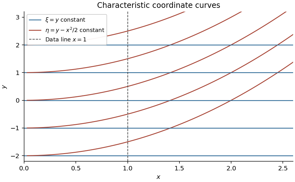
Writing $z(x,y)=Z(\xi ,\eta )$, the chain rule givesThe original equation reduces to $-x{Z}_{\eta }-x^3{Z}_{\xi \eta }=-x{Z}_{\eta }+x^3$, hence the canonical form is $\boxed{Z_{\xi \eta }=-1}$. Integrating once in each characteristic variable givesorOn $x=1$, differentiation gives $z_x=y-g^{\prime }(y-1/2)$. The specified derivative therefore forces $g^{\prime }=0$ for every argument, so $g$ is a constant. The specified value then gives $f(y)+g=1+y^2-y/2$. ConsequentlyIts derivatives are $z_x=xy$, $z_{xx}=y$ and $z_{xy}=x$, which verify both the equation and the data directly.

The Laplace transform isA sufficient condition is that $y$ be piecewise continuous on each bounded interval and of exponential order $c$, meaning $|y(t)|\le C{e}^{ct}$ for all sufficiently large $t$. Then the integral is absolutely convergent for $\mathrm{Re}p>c$, by comparison with $e^{-(\mathrm{Re}p-c)t}$.

For the constant function, direct integration gives

Combine the exponentials and integrate:The parameter $a>0$ makes this convergence half-plane larger than the one for the constant function.

Integration by parts, where the transform boundary term at infinity vanishes, givesFor a sufficiently regular function with the required exponential growth bounds, apply this again to $\dot{y}$ to deduceThese identities hold in a right half-plane where the displayed transforms converge; the regular solutions obtained below satisfy those requirements.

Differentiating the transform with respect to $p$ givesApplying this to $\mathcal{L}[1]=1/p$ also gives $\boxed{\mathcal{L}[t]=1/p^2}$ for $\mathrm{Re}p>0$.

Now put $Y=\overline{y}$, $y_0=y(0)$ and $v_0=\dot{y}(0)$. Transforming each term of the differential equation, and using the derivative identities, givesThe initial-value terms cancel, leavingIntegrating once yields $(p+1)Y=C+1/(2p^2)$. Partial fractions giveThe transform pairs therefore imply, on writing $A=C+1/2$,For the final parameter count, the differential equation is the derivative of $t(\dot{y}+y)$: it says $[t(\dot{y}+y){]}^{\prime }=t$. Integrating gives $t(\dot{y}+y)=t^2/2+B$. A regular solution at $t=0$ has finite $y$ and $\dot{y}$, forcing $B=0$. Thus $\dot{y}+y=t/2$ is first order and leaves only one constant. Equivalently, the original equation at zero requires $\dot{y}(0)+y(0)=0$, so the two usual initial values cannot be chosen independently. The displayed solution satisfies this constraint and verifies the original equation directly.