Original solutions to the paper released at the source request. The complete editable transcription is retained in the private examination archive.
The infinitesimal strain is . A constant translation has zero gradient. For the remaining term, has , a skew-symmetric matrix. ThereforePhysically is a translation and is an infinitesimal rigid rotation, with axis along and rotation angle . It is the linearized rotation displacement, not the exact displacement of a general finite rotation. This distinction matters because the infinitesimal strain omits quadratic displacement-gradient terms.
Choose zero energy in the unstrained state. The required strain energy density isIts variation is , giving the prescribed stress as the tensor gradient. This variational notation handles the symmetric off-diagonal components without a spurious factor of two.
Decompose into orthogonal deviatoric and spherical parts. ThenThe two squares vanish together only for . Thus and are sufficient for positive definiteness. They are necessary by testing a nonzero trace-free strain and a pure dilation separately. Equivalently both shear modulus and bulk modulus must be positive.
Multiply equilibrium by the displacement and integrate. Integration by parts and the traction condition giveThe stress is symmetric, so it contracts only with the symmetric part of , namely . Hooke's law then gives . HenceThe identity is the linear-elastic work balance: twice the stored quadratic energy equals the body-force and boundary-traction work paired with the final displacement.
Apply energy uniqueness for a linear elastic traction problem. Subtract two solutions with the same loading, writing their displacement difference as . Linearity makes its body force and boundary traction zero. The preceding energy identity therefore yields . Positive definiteness and continuity imply everywhere. By the permitted zero-strain characterization,Thus the solution is unique modulo infinitesimal rigid translations and rotations, on each connected body. Conversely adding such a displacement changes neither strain nor stress, so these are exactly the unconstrained modes. This is conditional uniqueness; existence of a pure-traction solution additionally requires balanced resultant force and torque.
Use the torsion stress function for a simply connected bar. The only nonzero strain components are and . ThusThe axial equilibrium equation is . Since the section is simply connected, the planar divergence-free stress field has a stream function:Equality of the mixed warping derivatives gives . On the lateral boundary the axial traction is , the tangential derivative of . Traction-free walls therefore make constant on the connected boundary, and its arbitrary additive constant can be chosen so .
Tresca's yield criterion requires the maximum shear stress, half the largest principal-stress difference, not to exceed the material's shear yield stress . The stress eigenvalues here are , so the maximum shear is andIf yield is instead quoted as a uniaxial tensile stress, that parameter is ; the present convention is the source's shear parameter.
For the ellipse, the proposed quadratic vanishes on its boundary. Its Laplacian fixesThe corresponding warping is . Elliptic polar coordinates , give , henceTo locate first yield, maximize . It increases radially to the boundary. For , the maximum there occurs at and equals . ThereforeThe positive-twist value is the requested expression. The ends of the minor axis yield first, not the ends of the longer axis. This is elliptical-bar torsion and first yield.
For an admissible variation with ,Stationarity for every variation therefore gives the Euler-Lagrange equationThe first energy term is bending energy: the curvature of an inextensible planar beam is . The shortening relative to the straight reference is . A prescribed compressive dead load does positive work on that shortening, so its potential-energy contribution is minus times that integral. A minimizer must satisfy the stationary equation, but a stationary solution need not be a minimizer.
Set . The endpoint interval becomes , and multiplication of the dimensional equation by givesThe energy in these variables is . Thus measures load relative to the first linearized eigenvalue for the angular endpoint conditions actually imposed.
Linearization gives . The two homogeneous Dirichlet conditions select . For any small trial amplitude in this mode, , soFor every nonzero quadratic variation is positive by the sharp Poincaré inequality. For , the first mode gives negative energy at sufficiently small amplitude, so zero cannot be a local minimum.
The printed strict “only if” conclusion omits the critical case. At the quadratic test is degenerate, not negative. In fact zero is still the unique minimum of the full displayed functional: use and to get , with strict inequality for a nonzero continuous function because when . In particular on the critical first mode,Thus strict positivity of the second variation holds for , while local minimality of the full energy holds also at . This is the distinction captured by critical-load minimality of the angular Euler strut.
Near the first eigenvalue, load detuning supplies a term , while the first nonlinearity in is cubic. Balancing them gives , so .
Put . At order ,The operator has kernel , so Fredholm solvability requires its forcing to be orthogonal to that function. Since and ,When this holds the nonresonant forcing is ; for instance is a solution after absorbing its arbitrary first-mode component into the amplitude convention.
The branches are . This is a supercritical pitchfork bifurcation. The leading reduced energy is proportional to : the nonzero branches are minima for , while zero loses minimality on that side. At the origin the quartic term still stabilizes the critical state.
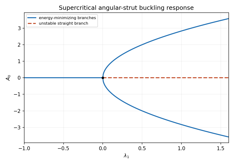
Supercritical strut response: stable nonzero branches emerge above the critical load; dashed zero branch is unstable
. Details. Take positive upwards, so the source's sign convention makes a downward applied load. The small-slope tension contribution on a short interval is . Let be the upward contact reaction. Force balance gives . Nonpenetration is , and reaction is absent where . ThereforeThe contact boundary must have continuous to avoid a broken string, and continuous slope in this smooth-contact model with no concentrated point force. Integrating force balance over a vanishing interval around a contact endpoint gives when the load and reaction are locally bounded. This is the one-dimensional obstacle problem, with its reaction acting as a nonnegative constraint force.
For any admissible , put . At endpoints . On the contact set, and imply , while away from contact the reaction is zero. Hence everywhere. Integration by parts givesRearranging proves the requested variational inequality. Piecewise integration is legitimate because the slope is continuous at the contact boundary, so there are no omitted point-force terms.
The small-slope excess length is , so the first term is the work needed against uniform tension. The second is the potential energy of the downward distributed load. Their sum is total potential energy subject to the obstacle constraint.
Expand the difference exactly:The first two integrals together are nonnegative by part (b), and the square is nonnegative. ThusFor this also proves uniqueness: equality for two minimizers forces identical derivatives, and the fixed endpoints remove their additive constant. The convex admissible set and strictly convex energy make the variational inequality a global minimization condition.
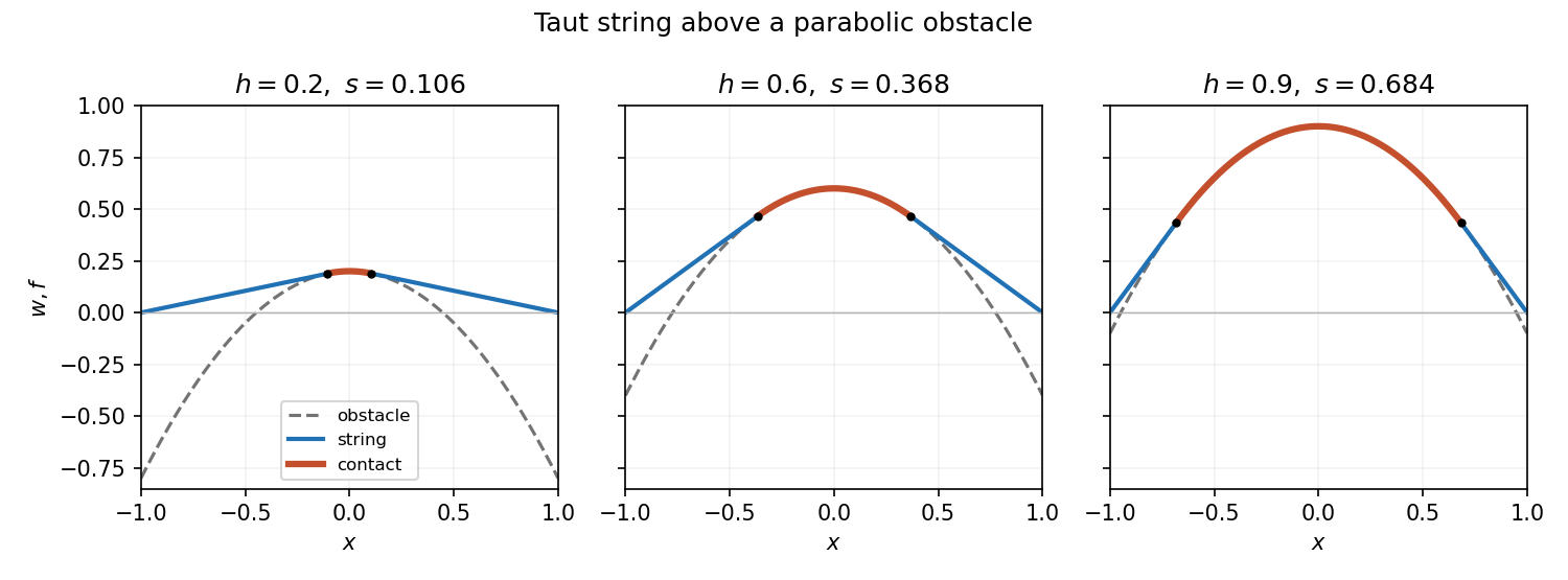
With no applied load the free string segments are straight, while in contact . By symmetry use contact and a right-hand line through tangent at . The tangency conditions are and , giving on and . ThereforeThe other algebraic root is outside the admissible contact interval except at the coincident endpoint .
Verification makes the construction complete: the values and slopes match at , the endpoints are zero, and outside contact . Inside contact ; outside it , so complementarity holds. The minimization argument proves this verified solution is the unique equilibrium. At the contact set is the single point and ; at contact fills the whole interval. This is the parabolic obstacle under a taut string.


Articles by others on the same topic
There are currently no matching articles.