Section V reuses the official solution notes, with PDF page numbers below counting the cover as page 1. Only omissions and a short correction are supplied here. Section VI is solved below. The examiner report supplies feedback, rather than a worked answer set.
The official notes, PDF p. 7, handwritten p. 1 derive the affine choice of coordinate time and the circular-orbit angular velocity from the geodesic equations.
The official notes, PDF pp. 7–8, handwritten pp. 1–2 calculate both elapsed proper times and their weak-field ratio for satellite A and the polar station.
The official notes, PDF pp. 8–9, handwritten pp. 2–3 calculate the geostationary satellite/station proper time ratio, including the equatorial station's rotation. They explicitly correct the formula printed in the paper; the printed target is not the first-order result of the stated Schwarzschild metric.
The official notes, PDF p. 9, handwritten p. 3 compare the two clock ratios and identify the station's rotational contribution. PDF p. 10, handwritten p. 3a, separately clarifies the normalization when coordinate time is the affine parameter.
The official notes, PDF pp. 11–13, handwritten pp. 4–6 derive all four geodesic equations and list the twelve nonzero Christoffel symbols up to symmetry of the lower indices, using time coordinate .
The official notes, PDF pp. 13–14, handwritten pp. 6–7 integrate the radial geodesic equations and establish the vanishing integration constant for a null geodesic.
The official notes, PDF pp. 14–16, handwritten pp. 7–9 integrate the exponential scale factor, discuss the sign required for an incoming photon, and obtain the distance–redshift relation. They use for the paper's otherwise undefined .
The official notes, PDF pp. 17–18, handwritten pp. 10–11 give the matter density, curvature and cosmological constant scalings and the requested logarithmic sketch. For the closed model the curvature contribution to the Friedmann equations is negative; the sketched curvature magnitude must be read with that sign restored.
The official notes, PDF p. 18, handwritten p. 11 explain the imminent maximum expansion, recollapse, remaining time of order the present age, and total lifetime of approximately twice that age.
The official notes, PDF p. 19, handwritten p. 12 integrate the radial null geodesic, express the radial coordinate in terms of comoving distance, and give its maximum value in that coordinate chart. The maximum radial coordinate is not the total path length around a closed spatial slice.
The official notes, PDF pp. 20–21, handwritten pp. 13–14 combine the Friedmann equations and Raychaudhuri equation to derive the density and scale factor of the Einstein static universe.
The official notes, PDF p. 21, handwritten p. 14 give the acceleration signs and the instability conclusion for the Einstein static universe. One wording correction is necessary: their word “oscillatory” for the overdense perturbation is a slip. Starting near rest, an overdense model contracts and its matter density rises, whereas an underdense model expands and its matter density falls; both move away from the static balance.
The official notes, PDF pp. 22–23, handwritten pp. 15–16 give both density scalings, integrate the radiation- and matter-dominated Friedmann equations, normalize the late solution today, and match the two approximations at equality.
The official notes, PDF p. 24, handwritten p. 17 integrate the physical particle horizon and derive its early-time redshift dependence, explicitly stating the present matter-dominated approximation used in the printed expression.
The official notes, PDF pp. 24–27, handwritten pp. 17–20 obtain the photon number density by integrating the Planck distribution, explain the temperature and dilution scalings, and compare the interaction time with the expansion time for thermal equilibrium. They also correct the missing cube and factor-of-two error in the paper's printed photon number density.
The official notes, PDF p. 27, handwritten p. 20 derive the early-time photon count, its vanishing limit, and the failure of thermal equilibrium when the count is of order one. Two details need supplementing.
First, their constant is the normalization obtained by extrapolating the early-time particle horizon formula to . It is not the count within today's actual particle horizon. Let and let be that horizon's physical radius. Using the paper's early-time approximation givesFor a present matter-dominated approximation, . Alternatively, retaining both components in the flat model exactly, , and integrating the particle horizon givesThe second boxed formula uses the exact two-component normalization and the radiation-dominated early-time limit. Its large- leading term agrees with the first expression and .
Second, a particle horizon containing only order-one photons cannot support a smooth, locally representative radiation density: discrete-particle fluctuations are of the same order as the mean, and a single photon's direction is strongly anisotropic. Thus the fluid description assuming spatial homogeneity and cosmological isotropy is not self-consistent on that causal scale. This does not by itself disprove an ensemble-averaged cosmological symmetry; it limits the extrapolation of the smooth thermal equilibrium description.
For the mutually orthogonal direct primitive lattice translation vectors , define the reciprocal lattice basis byThus , with integer , satisfies for every lattice vector .
Write . The electron density is periodic with period one in each , so its three-dimensional Fourier series has integer harmonics:If is a primitive unit cell of volume , Fourier orthogonality givesConversely, translation by multiplies a general plane wave by . Periodicity permits only , precisely the reciprocal lattice vectors. For a physical bounded periodic electron density, the expansion exists in the usual square-integrable sense.
Use the scattering vector ; reversing its sign conjugates the following amplitudes without changing the intensities. In the kinematic approximation, the atomic scattering factor of atom isAtoms at therefore give the scattering amplitudeHere is the single-electron amplitude; is the unit cell structure factor, and is the geometrical lattice sum. If the crystal has repeats along , the latter factor is a product of geometric series, whose magnitudes containThe sharp constructive peaks occur when every . Thus a permitted reflection has wavevector change equal to a reciprocal lattice vector, with and the additional elastic condition . A finite crystal broadens these peaks; it does not impose an exact delta-function selection on every scattered photon.
In the conventional cubic unit cell, the four face-centered cubic lattice positions contributeThe two-atom atomic basis of a crystal gives the zinc blende structure factorMixed-parity Miller indices have . With all indices even or all odd, . For real atomic scattering factors,Hence all same-parity reflections are generally permitted in GaAs, although the last class is weak when the two atomic scattering factors nearly coincide. These are the structural selection rules; a particular experiment must also satisfy the elastic Bragg scattering condition.
In the electron-count estimate , , the structure factors are and . Thus a single-directed-reflection estimate isA powder X-ray diffraction peak collects all equivalent reflections. The powder diffraction multiplicities are eight for and six for , so the multiplicity-and-electron-count estimate isAt the two sublattice amplitudes are opposite in phase and nearly cancel; at their relative phase is a quarter cycle, so this cancellation does not occur. In silicon, the two atomic scattering factors are identical and the diamond cubic structure has an exactly forbidden reflection, while remains allowed in the kinematic approximation.
The numerical ratio neglects the angular dependence of the atomic scattering factors, the Lorentz-polarization factor and thermal-motion corrections. No wavelength or measurement geometry is supplied to refine those factors. This is therefore a stated structural estimate, rather than a unique precision ratio of measured peak areas.
Let be a stable equilibrium separation: , . With bond extension , the Taylor expansion isThe harmonic approximation applies when the typical thermal and zero-point bond fluctuations satisfy and the higher terms are negligible, for example and . The relevant small quantity is the relative displacement of neighbouring atoms. Small bond excursions about a stable minimum give an amplitude-independent spring constant . Large thermal excursions, bond breaking or appreciable anharmonicity invalidate the approximation.
With atomic displacement , the harmonic potential energy is . Newton's second law givesFor a periodic chain of atoms, its normal modes are , with and one representative per Brillouin zone. Substitution yields the monatomic-chain dispersion relationA real general displacement is a superposition of these normal modes and their complex conjugates. The mode is a rigid translation. At small , the acoustic phonon branch is linear, with speed of soundFor , the group velocity is and vanishes at the zone boundary. The dashed initial tangent in the sketch has slope .
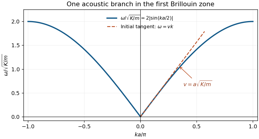

For the Lennard-Jones potential,Its minimum and harmonic spring constant areUsing the monatomic-chain dispersion relation,The maximum is at . Taking the argon atomic mass as and givesThese are the stipulated one-dimensional nearest-neighbour model estimates; a three-dimensional argon crystal has additional neighbours and phonon polarizations.
Normalize the plane waves in a periodic crystal of area or volume . The Fourier coefficients of the periodic potential obeyTranslation of the integral by any lattice vector leaves it invariant but multiplies it by . A nonzero result therefore requires to be a reciprocal lattice vector.
Near an isolated Bragg scattering degeneracy, ordinary nondegenerate perturbation theory fails because the free energies coincide. Retain the resonant plane waves , and apply degenerate perturbation theory. Absorb the constant into the energy origin. Since a real potential has , the projected Schrödinger equation has coefficient matrixA nonzero eigenstate requiresOff-resonant plane waves give higher-order energy shifts omitted in this leading nearly-free electron model.
Let andAt the two degenerate plane waves have momenta and and coupling . ThusTheir symmetric and antisymmetric combinations are the lower and upper states respectively. The local band gap is .
Put . At , the free energy is . The four cyclic combinations in the supplied secular equation give the four-plane-wave splitting at a square-zone cornerFor example, the normalized coefficient vectors in the source's cyclic basis are , , , and . Because , these are ordered as written: a lower singlet, a central doublet and an upper singlet. The sketch puts the and energies on one common scale; its representative negative couplings are stated in the caption.
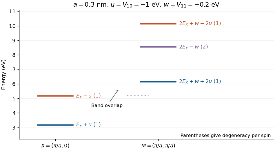
Common energy scale at the square-zone edge and corner, with illustrative couplings V10 = −1 eV and V11 = −0.2 eV
. Details. 
There are two electrons per primitive unit cell; a spin-degenerate energy band accommodates exactly that number. A semiconductor results when the first band is full and does not overlap the second. In the leading two-wave/four-wave approximation, compare the first-band maximum at with the second-band minimum at :This is an indirect band gap; a nonzero local splitting at alone is insufficient. At the onset,With , gives , henceFor more negative than this value the estimated indirect band gap is positive; at equality the bands just touch. This is the onset estimate within the source's nearly-free electron model truncation, not an exact critical potential after coupling all plane waves.
The Brillouin function is odd, increases monotonically through zero, and approaches for . Its small- slope is . For , the magnetic ions overwhelmingly occupy the largest field-aligned moment projection, so the magnetization reaches magnetic saturation:The sketch shows several values; all have the same limiting values, while their slopes differ.
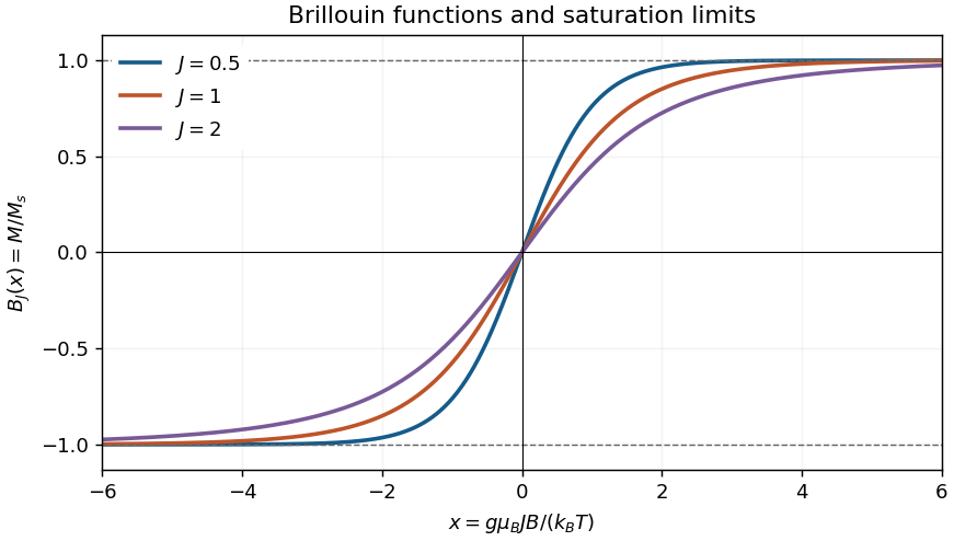
Brillouin functions approaching magnetic saturation
. Details. 
The terms in the Brillouin function cancel. Keeping the linear terms givesConsequently,Use the dimensionless SI magnetic susceptibility and , as in the source's molecular-field convention. The Curie law isIf susceptibility is instead defined as , its coefficient is and is dimensionful. The SI convention above makes the subsequent Curie–Weiss law and consistent.
For positive , a fluctuation of magnetization produces a Weiss molecular field in the same direction, reinforcing alignment. The mean-field self-consistency equation isLinearizing in the paramagnetic phase givesAt zero applied field, the right-hand side's slope at is . Below this exceeds one, and the saturation of the Brillouin function allows stable nonzero solutions of opposite sign: spontaneous ferromagnetism. Above , only the zero-field solution remains stable. The stated linear susceptibility is the paramagnetic branch for ; it must not be continued as a negative susceptibility below the transition.
Using the supplied iron parameters givesAn internal Weiss molecular field depends on temperature through . Its low-temperature saturation estimate uses :At and above the zero-applied-field magnetization vanishes in this model, so this is a saturation estimate, not the field at .
Use the paper's stipulated face-centered cubic lattice, which has twelve nearest neighbours. The saturated one-ion alignment scale isDividing the effective field among twelve equivalent neighbours gives the per-bond exchange interaction scaleTo specify the convention, write the Heisenberg model as , with dimensionless angular-momentum operators and each bond counted once. Then , so here. A convention with instead has . The total saturated interaction energy per ion is ; the factor of one half avoids counting each bond twice.
Articles by others on the same topic
There are currently no matching articles.