Original paper: Public original PDF, physical pages 25–33; question pages 26–33.
A Bravais lattice is a set of equivalent points generated by integer combinations of three independent translation vectors. A crystal motif is the arrangement of atoms attached identically to every lattice point. Together they specify the periodic crystal structure: lattice translations repeat the motif without changing its internal arrangement.
A unit cell is a region whose translations tile the structure. A primitive unit cell contains one lattice point after sharing boundary points with neighboring cells. A conventional cell can contain more than one lattice point to display the crystal's symmetry with simple axes and angles; for example, a conventional face-centered cube has four lattice points but a less visually symmetric primitive cell has one.
Rotational symmetry compatible with a periodic three-dimensional lattice has order or , as expressed by the crystallographic restriction theorem. A crystallographic fivefold axis is excluded from an ordinary periodic crystal. This statement concerns exact lattice symmetry; it does not exclude local fivefold atomic arrangements or nonperiodic ordered structures.
The body-centered tetragonal lattice has points at and in the conventional cell. Add the two-atom motif to each. Reducing coordinates modulo integer translations givesThus the cell contains four atoms, not merely the two lattice points. In projection along , label each projected point by its fractional height ; the four sites do not all lie in the same plane.
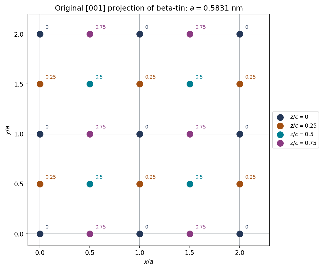
Original calculated projection of two-by-two conventional beta-tin cells; colors and labels give fractional height, not different chemical species
. Details. 
The plotted repeat is in both horizontal directions. Atoms on the outer drawing boundary are repeated images needed to show neighboring cells, rather than additional unshared atoms in the four-cell counting volume.
The metallic conventional cell has four tin atoms, whereas the conventional diamond cubic structure cell has eight. Therefore the volume per atom isThe fractional change for metallic to nonmetallic tin isThe atom count is unchanged, so this is also the unconstrained bulk volume change for complete transformation under the model. If it were macroscopically isotropic, the corresponding free linear expansion would be .
Such a large transformation strain creates stresses where transformed and untransformed regions constrain one another. Cracking, loss of mechanical integrity and disintegration can follow: the phenomenon is tin pest. The calculation establishes the volume mismatch, not the transformation rate; temperature, nucleation and impurities affect when a real specimen changes.
The 020 reflection is extinguished by the diamond basis, even though it satisfies the face-centered lattice parity rule. Write the diamond structure as an FCC lattice with identical atoms at basis positions and .
The structure factor separates into lattice and basis terms:At , all indices are even, so the first bracket is . The second bracket is . The two identical sublattices scatter with opposite phases and cancel:For all-even reflections of diamond, the additional allowed condition is divisible by four. This is a systematic absence, not an absence of the corresponding family of geometrical planes.
The voltage is a mechanically mediated effect: nickel magnetostriction strains the bonded central layer, and the direct piezoelectric effect converts stress into electrical displacement. An estimate of requires a strain-transfer and electrical-boundary assumption.
Let run along the applied field and through the layers. Assume saturated, approximately volume-preserving isotropic nickel magnetostriction, perfect bonding, mechanically dominant nickel faces and a high-impedance voltage measurement. Relative to the random-domain state,Treat the thin central layer as in plane stress, with these imposed in-plane strains, negligible converse-effect backreaction and isotropic elastic constants. ThensoFor a transversely polarized layer,The open-circuit increment has , and . HenceThe observed voltage magnitude does not specify the sign without electrode polarity and poling direction. A one-dimensional approximation retaining only axial stress instead gives . That is a different mechanical model. Nickel stiffness and thickness, interface compliance, central-layer tensor coefficients and electrical loading are not specified, so the experiment does not determine a unique exact intrinsic coefficient without these assumptions.
For a conventional initially random, untextured piezoceramic, orientational averaging suppresses the macroscopic linear response. Electrical poling of ferroelectric domains is the usual way to generate a lasting net response. Under that conventional preparation assumption, a ferroelectric constituent is the expected route.
However, the word polycrystalline alone does not logically require ferroelectricity. A deliberately textured aggregate of nonswitchable piezoelectric grains can have a nonzero effective tensor if their orientations and polar directions do not cancel. Ferroelectricity means electrically switchable spontaneous polarization, whereas piezoelectricity means linear stress–charge coupling. Thus the unconditional statement that every polycrystalline piezoelectric must be ferroelectric is too strong.
No. A piezoelectric single crystal need not be ferroelectric. A noncentrosymmetric crystal can couple strain to polarization without having a spontaneous polarization that an electric field can switch. Quartz is a standard example.
A single crystal already has an oriented crystallographic tensor, so the random-grain cancellation issue does not arise. The relevant tests are crystal symmetry and the nonzero piezoelectric coefficients; ferroelectric switching is a separate property.
If removal restores the original random-domain magnetic state, the magnetostrictive strain and induced voltage return toward their original values. Elastic strain transfer then relaxes the stress on the central layer.
A ferromagnetic nickel layer can retain remanent magnetization and an altered domain population, so removing the external field does not guarantee removal of all magnetostriction. The electrical time response also depends on leakage and the input impedance of the voltmeter: an open-circuit strain-induced voltage can decay through a finite resistance even while some strain remains. The final observed voltage is therefore history- and circuit-dependent.
Reversing a saturating longitudinal field gives approximately the same strain and the same voltage polarity relative to the original unmagnetized reference. In the isotropic orientational model,It is unchanged under . Both positive and negative longitudinal saturation therefore contract the negative-magnetostriction nickel in the same axial direction. The resulting stress on the piezoelectric layer has the same sign.
During field reversal there can be a hysteretic transient as domains reorganize, and finite circuit leakage can alter the measured waveform. Those effects do not turn the saturated strain law into a response odd in the field.
Assume that the transverse field is large enough to saturate through the thickness despite demagnetizing effects, and retain the thin-layer plane-stress and open-circuit assumptions from part(a). The two imposed in-plane strains now becomeTheir sum is , whereas it was for longitudinal saturation. The in-plane stress sum, and hence the induced open-circuit voltage, is multiplied by :Thus the magnitude is about with the opposite polarity, under this model. The larger demagnetizing field for an out-of-plane direction means the same external field magnitude might not produce the same degree of saturation. Changes in thickness constraint or strain transfer would also modify the estimate.
For a cubic phase, and Bragg's law givesThe first six FCC-allowed squared-index sums are , from indices all odd or all even. The labels1–6 are thereforeRemember that the plot reports , not . The first peak givesThe last peak provides an independent estimate,Thus is appropriate to the supplied precision. The two estimates differ by about ; high-angle data are less sensitive to a fixed angular error, so the estimate is useful for the composition calculation. The printed angles do not justify many more significant figures or an exact fit of all six positions.
Sample A is the Cu–Au alloy. At the indicated copper-rich composition, the supplied Cu–Au diagram permits one copper-rich solid-solution phase. The Cu–Ag diagram instead gives two equilibrium solid phases at room temperature. A single consistent set of FCC peaks therefore identifies A under the stated equilibrium assumptions; similar pure-metal lattice parameters alone would not distinguish gold from silver.
Use Vegard's law as an approximate atomic-fraction interpolation:With the higher-angle estimate from part(a),This is about atomic percent, not weight percent. Using rounded molar masses and ,Using the first peak alone instead gives roughly . The justified conclusion is therefore about – gold, with uncertainty from angle rounding, calibration and the approximate linear lattice-composition relation.
Sample B should show two FCC peak families, one from a copper-rich phase and one from a silver-rich phase. Their lattice parameters are set by the compositions of the coexisting phases, not by one lattice parameter at the overall alloy composition.
For corresponding Miller indices the silver-rich phase has a larger lattice parameter and hence a larger interplanar spacing, so its reflection occurs at smaller . Some reflections may overlap or be weak. Relative intensities depend on phase fractions, atomic scattering factors, absorption and texture; a raw peak-height ratio is not directly a mass fraction.
At room temperature the mutual solubilities in the supplied Cu–Ag diagram are small, so the two families would be near the elemental copper and silver positions. Slow cooling is important: a metastable supersaturated single phase would be a different interpretation. Quantitative phase or composition analysis would require calibrated diffraction and an appropriate refinement, not merely counting the visible peaks.
SEM with energy-dispersive X-ray spectroscopy can identify gold versus silver through their characteristic X-ray energies. Acquire spectra and maps from representative regions: two compositionally distinct regions would support the two-phase interpretation of B. With standards or validated matrix corrections it can estimate local compositions and, with representative sampling, an overall composition. Surface topography and the interaction volume limit spatial interpretation.
X-ray fluorescence provides a complementary more bulk-averaged elemental measurement. Gold and silver produce different characteristic lines; calibrated intensities can yield their mass fractions, with corrections for absorption, excitation and specimen geometry. It does not by itself determine whether an element occupies one or two crystallographic phases.
Both methods supply elemental information missing from a lattice-parameter-only identification. A purely morphological micrograph could reveal phase separation but would not alone give a reliable numerical chemical composition.
Pearlite is a microstructural arrangement of two phases, ferrite and cementite, rather than a single phase. Ferrite is an iron-rich solid solution; cementite is the carbide . A pearlite colony contains alternating lamellae of these constituents formed by transformation of austenite.
A thermodynamic phase has a specified crystal structure and composition range with locally homogeneous properties on the appropriate scale. The word pearlite instead describes how distinct phases are arranged. Its lamellar spacing and orientation can change while the identities of its two phases remain the same.
Use the line fraction occupied by the tall narrow ridges as an estimate of cementite volume fraction, assuming the line is representative and its etched height classification identifies the phases correctly. The displayed profile gives roughly cementite and ferrite.
An operational measurement at a height threshold near gives four ridge widths totaling about over a profile about long:Changing the threshold over a reasonable part of the high ridges gives roughly –, so this is an image-based estimate, not an exact phase analysis. The occasional low protrusions should not all be counted as full cementite lamellae merely because they are above a noisy baseline. The reference line and threshold convention must be stated.
For eutectoid pearlite, apply the lever rule between ferrite and cementite at the transformation temperature. Using standard approximate Fe–C values , and in weight percent carbon,These are mass fractions. To compare with an unbiased geometric line fraction, convert using the phase densities:With representative densities and , this gives about cementite and ferrite. Because the densities are similar, the mass and volume fractions differ only modestly. The phase-diagram values here are conventional approximations, not a claim that the exact 2018 Data Book has been recovered.
The profile estimate and equilibrium lever-rule estimate need not agree exactly. The height trace contains only four major ridges, making it a small sample of the microstructure. Pixel size, ridge-threshold choice, tip geometry, contamination, polishing damage and unequal etching change apparent widths. A finite-radius AFM tip can broaden the narrow raised cementite regions, biasing their inferred fraction upward.
The equilibrium calculation assumes eutectoid pearlite with the chosen carbon composition and tie-line values. Off-eutectoid steel can include proeutectoid ferrite or cementite outside the pearlite; alloying, carbon segregation and non-equilibrium cooling alter the simple Fe–C estimate. Carbon solubility also varies with temperature. The mass-to-volume conversion requires phase densities.
The observed difference between roughly ridge fraction and equilibrium phase volume is therefore a reason to examine sampling and the etched-surface measurement, not to force the image widths to match the lever rule. Multiple colonies, repeated calibrated traces and a phase-sensitive measurement would improve the comparison.
Ferrite etches faster in Nital, so it recedes and leaves cementite standing as the higher ridges. The identification is based on the surface-relief preparation, not on assuming that every bright feature in every microscopy mode is cementite. In the stated AFM image, brightness is a displayed height contrast.
The lamellar interfaces now make with the surface normal, or with the surface itself. Draw inclined alternating plates rather than vertical stripes, with preferentially etched ferrite below the more resistant cementite.
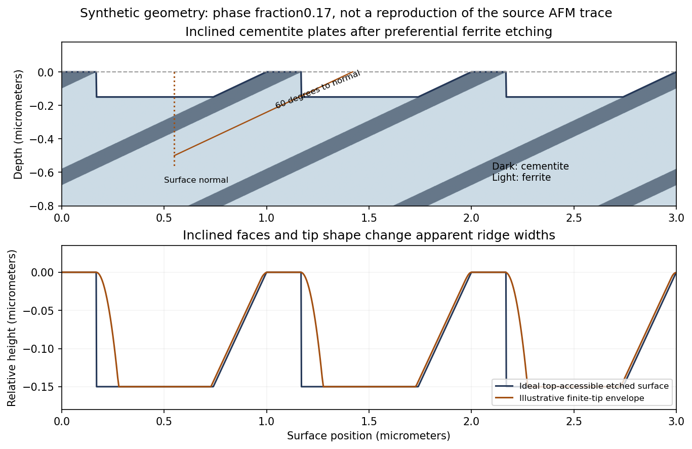
Original inclined-lamella etching geometry and illustrative AFM profile; the synthetic spacing and fractions are not a tracing of the source data
. Details. 
The upper panel shows an inclined microstructure intersecting the original plane. Differential etching can expose a shallow inclined cementite face on one side of a ridge and an undercut or overhang on the other. The lower panel shows its accessible height profile, with additional rounding from a finite tip. It is therefore possible to obtain an asymmetric ridge even from an initially planar section through parallel lamellae.
For an ideal unetched planar cut, a plate of normal thickness has apparent surface widthThe same factor applies to the ferrite spacing. Inclination alone broadens all intersections together; it does not by itself change the true phase-width ratio.
The danger is identifying an etched height interval with the original planar phase intersection. Preferential ferrite dissolution exposes inclined cementite faces and can produce overhangs. A conventional AFM tip cannot follow a reentrant underside; its finite size also broadens ridge tops and may not enter the intervening troughs. A thresholded height width can consequently differ from both the true plate thickness and its original surface intersection.
A uniform inclination at an ideal flat cut does not itself invalidate a line-fraction estimate: both phases acquire the same geometrical width factor, which cancels in their ratio. The problem is differential relief and probe accessibility after etching, together with uncertain local angles and limited sampling. Using only the apparent ridge occupancy can overestimate cementite. An independently polished section, calibrated probe geometry, several directions and colonies, or another phase-sensitive method is needed to test the inference.
Assume a thin cylindrical wall, uniform internal pressure and closed ends carrying the pressure load. The radial stress is small compared with the membrane stresses when .
For an end cap, the outward pressure force is . The wall's axial tensile force is . Equilibrium therefore givesFor a longitudinally split half-cylinder of length , pressure has resultant across the projected rectangular area. Two cut wall sections each carry , soThus hoop stress is twice the closed-end axial stress in this model. An open-ended tube without an external end load does not acquire the same pressure-induced axial membrane stress.
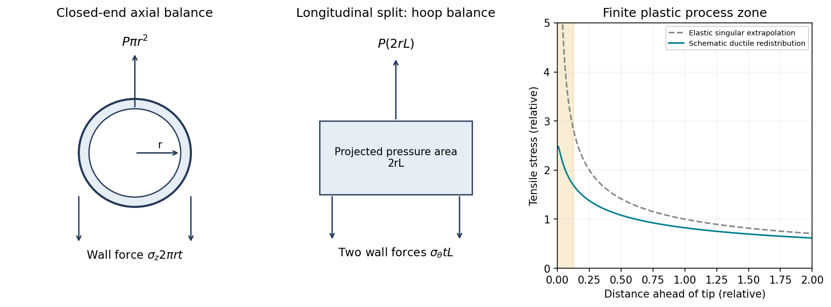
Original thin-pipe force balances and schematic crack-tip stress regularization by plastic deformation; the plastic-zone curve is qualitative
. Details. 
Linear elastic fracture mechanics predicts a near-tip tensile stress varying approximately asA ductile material yields near the tip before that mathematical singularity can be realized. Plastic deformation blunts the crack and redistributes stress over a finite process zone, as shown in the right-hand diagram. Constraint can sustain stresses above the uniaxial yield stress, so the schematic plateau should not be interpreted as a universal exactly- cap.
A useful process-zone scale is with a geometry- and constraint-dependent coefficient. Advancing the crack then requires energy for plastic deformation and other irreversible processes as well as forming new surfaces. Consequently the critical energy release rate is much larger than the reversible surface-energy term of a perfectly brittle idealization:In a small-scale-yielding plane-strain description, with . Large-scale yielding requires an elastic-plastic measure rather than treating a linear-elastic stress-intensity criterion as exact. The increased dissipation and crack-tip blunting explain the larger energy requirement.
Let be a characteristic crack depth and its geometry factor. A simple fast-fracture condition isThe crack should penetrate a wall of thickness before reaching the critical size, so the simplified leak-before-break criterion is , with appropriate geometry and stable-through-wall-crack assumptions.
The conventional material-based maximum thickness uses the yield stress as a conservative limiting operating stress:It ensures that the depth required for penetration is subcritical even at the stated limiting stress. Geometrical factors depend on crack shape and orientation; this is an educational screening estimate rather than a full crack-growth or leak-detection analysis. The handbook's fracture formula uses the same stress-intensity and geometry-factor convention.[ref]
Materials Data Book by Cambridge University Engineering Department. 2011 edition revised2019, printed p.6, Fast Fracture; this confirms the formula convention, not the exact2018NST supplied values
There is an important distinction if the actual pressure and radius are fixed while thickness varies. Substituting at penetration givesThat is a lower, not upper, bound on thickness under the fixed-pressure model. Yield avoidance additionally requires . It would be inconsistent to derive the fixed-pressure expression and call it a maximum. The standard maximum quoted above answers a different, yield-limited material-selection comparison.
For the aluminium alloy, write and for the appropriate data-book properties at the relevant material state and temperature. The yield-limited screening bounds from part(c), with , areFor in and in , the numerical substitutions are and .
A high-strength alloy's large yield stress can require a small allowable leak-before-break thickness even when its minimum pressure thickness is modest. FCC structure generally favors low-temperature plasticity, but does not by itself establish the alloy's fracture toughness, weld performance, corrosion behavior or fatigue resistance.
TODO: exact numerical thickness pending the identified 2018 NST Data Book values and alloy condition. The accessible Engineering2011/revised2019 book is not confirmed as the supplied edition; generic aluminium property ranges are not substituted as if they were the exam's values.
For Ti–6Al–4V, use its own fracture toughness and yield stress inThe same unit-conversion formulas from part(i) apply. A feasible yield-limited screening interval requires , using consistent crack geometry and low-temperature properties.
High specific strength and corrosion resistance can be attractive, but cost, fabrication, joining and toughness must also be assessed. The label HCP is not a sufficient rule that every titanium alloy has the same sharp ductile-to-brittle transition as ferritic steel; actual low-temperature alloy and microstructural data are needed.
TODO: exact numerical thickness pending the 2018 NST Data Book's Ti–6Al–4V property pair. No historical value or material-specific Arctic toughness is invented.
For mild steel, the corresponding bounds areA relatively low yield stress increases the thickness needed to carry pressure, but a favorable toughness-to-yield-strength ratio can give a much larger leak-before-break upper bound. This tradeoff often makes a tough structural steel more attractive than choosing the highest strength alone.
For Arctic service, the ductile-to-brittle transition is crucial. A room-temperature toughness cannot be assumed to persist below the transition, and welding, constraint and loading rate affect the comparison. A suitably qualified low-temperature steel can be practical; the word mild alone does not establish that qualification.
TODO: exact numerical thickness pending the 2018 NST Data Book values. The temperature and state of the tabulated toughness must also be identified before making a numerical service claim.
For high-strength steel, useAt fixed toughness, raising yield stress reduces quadratically but reduces the required pressure thickness only linearly. Thus a higher-strength grade can have a worse leak-before-break screening margin. The relevant screening combination is , since simultaneous satisfaction requiresUse measured low-temperature toughness and appropriate joining/environmental performance; strength alone does not establish suitability. The comparison also has to remain within the thin-wall approximation.
TODO: exact numerical thickness pending the 2018 NST Data Book's high-strength-steel property pair. The four material rankings cannot be made numerically definitive from the exam PDF alone.
TODO (user-deferred biology): this protein-rubber subpart is not researched or solved in the current nonbiology scope.
TODO (user-deferred biology): this protein-rubber subpart is not researched or solved in the current nonbiology scope.
TODO (user-deferred biology): this protein-rubber subpart is not researched or solved in the current nonbiology scope.
Interpret the supplied real quantity as the storage modulus , with the spring modulus in this continuum representation and the corresponding viscosity. Let . ThenAt high frequency, , the response approaches the spring stiffness; at low frequency it becomes much softer:In the series Maxwell model, the spring and dashpot carry the same stress while their strains add. A rapidly changing load allows little viscous flow, so the spring dominates the strain response. Over a long cycle the dashpot has time to deform, giving a small storage modulus and a fluid-like low-frequency response. This is generic viscoelastic mechanics, independent of the biological parts deferred above.
With , the curve isIt rises linearly from zero, bends downward and approaches the plateau . Its half-height occurs at .
For , the dashpot contributes the larger strain and dominates the compliant response. For , dashpot deformation during a cycle is small relative to spring strain, and the response is spring-dominated. The crossover separates these regimes rather than a discontinuous transition.
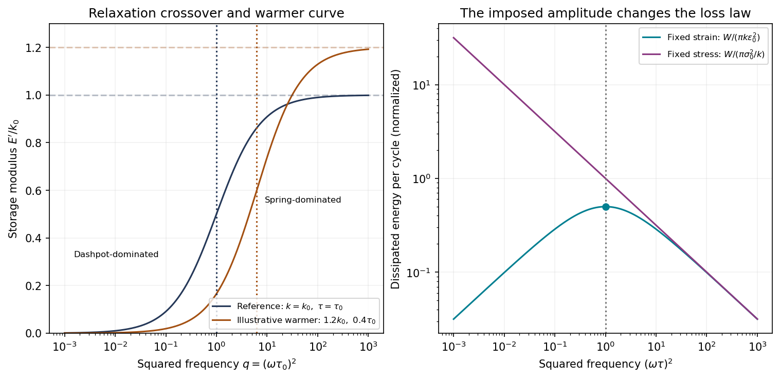
Original Maxwell storage curves versus squared frequency and the distinct dissipation laws at fixed strain and fixed stress amplitudes; axes use logarithmic spacing to show both regimes
. Details. 
The conventional relaxation-loss peak near applies to fixed strain amplitude, not to fixed stress amplitude. This distinction matters because the question explicitly describes oscillating stress.
The full complex modulus of the series Maxwell element isFor imposed strain , the energy dissipated per volume per cycle isSince has its maximum at , fixed-strain loss per cycle peaks at . At that scale the imposed cycle time is comparable with the relaxation time, and substantial viscous flow occurs while stress remains appreciable.
For the literally stated comparison with fixed stress amplitude, use the complianceThe dashpot strain rate is . Its dissipation integrated over a period givesThis decreases monotonically with frequency; there is no finite-frequency maximum at fixed stress amplitude in the ideal Maxwell model. Its mean dissipated power is , independent of frequency. The formal low-frequency divergence in energy per cycle accompanies very large strain excursions and cannot be extrapolated beyond the linear model's range. The graph identifies both results rather than assigning the fixed-strain peak to the wrong loading condition.
Within the rubbery regime, viscosity usually decreases as temperature increases, because segmental rearrangement becomes easier. The spring's entropic contribution generally increases approximately with absolute temperature at fixed effective network density, so tends to increase modestly under that assumption.
Consequently decreases. The storage-modulus crossover moves to larger squared frequency,and the high-frequency plateau moves upward if increases. The warmer curve in the figure illustrates those two changes. At intermediate frequencies the reduced relaxation time can lower the storage modulus even though its eventual plateau is higher; there is no requirement that the entire curve move upward.
These trends assume the same rubbery material state and no degradation, crystallization or change in effective network density. Close to other transitions the simple entropic-spring and viscosity picture needs modification.
A displacive transformation changes structure through coordinated atomic displacements, whereas a reconstructive transformation changes the bonding/connectivity arrangement more substantially.
In a displacive change, neighboring atoms move cooperatively without the long-range compositional redistribution characteristic of diffusion-controlled precipitation. The change can preserve many near-neighbor relationships and can occur rapidly when its kinetic conditions are met.
A reconstructive change requires breaking and re-forming the relevant structural connections to establish a different arrangement, often with a larger activation barrier and slower nucleation and growth. It may consequently show substantial kinetic persistence of a metastable phase. The distinction concerns the atomic mechanism, not merely whether the final phase has a different symmetry; neither label by itself supplies a universal transformation rate.
For two phases of the same pure substance at equilibrium, their chemical potentials are equal. Along their coexistence boundary,Differentiating the equality givesTherefore the Clapeyron equation isMolar or mass-specific quantities give the same slope if a consistent basis is used. follows from equal Gibbs free energies at coexistence.
Solid phases are relatively incompressible and have modest thermal expansion over many intervals. If their entropy and volume differences vary slowly enough that is approximately constant, the boundary is approximately straight. Straightness is an approximation, not a thermodynamic requirement. Heat-capacity differences, pressure dependence of volume, other transitions and proximity to special points can curve the boundary. The ideal-vapor integrated Clausius-Clapeyron approximation is not appropriate for these two solid phases.
Read the coesite–stishovite boundary at approximately and . The slope is thereforeA Celsius temperature difference equals the corresponding kelvin difference. The graph does not justify treating the endpoints as exact measurements.
For stishovite, the tetragonal cell volume divided by two givesFor monoclinic coesite the cell volume is , soUsing and Avogadro's constant, the mass-specific volumes areFor the direction stishovite to coesite,For the reverse, coesite to stishovite, the entropy change is about . Stishovite is the denser phase: a positive boundary slope and its smaller volume imply a lower entropy on the high-pressure side. Stating the direction prevents an otherwise avoidable sign ambiguity.
Articles by others on the same topic
There are currently no matching articles.