Original solutions to the paper released at the source request. The complete editable transcription is retained in the private examination archive.
The left side is atmospheric heat storage per unit surface area. Incoming solar flux is averaged over the spherical surface by the factor ; albedo reflects a fraction of it. The outgoing term is a reduced Stefan-Boltzmann flux, with effective emissivity representing atmospheric greenhouse trapping. Ice-albedo feedback usually makes decrease as temperature rises through an ice-melting range; greater carbon-dioxide pressure increases infrared opacity and therefore decreases this effective . The simple estimates below hold albedo fixed.
Radiative equilibrium givesDifferentiating gives . A doubling from Pa changes pressure by Pa, henceReference weathering balance requires , so .
For the requested approximate system, take as the reference radiative/weathering equilibrium, set , , and , whereLinearize the radiative loss, retaining terms linear in and . Its two terms are and . The carbon balance scales exactly with . ThereforeNumerically . The time conversion uses seconds for the radiative constants and years for the supplied carbon production.
Because , temperature rapidly approaches , while carbon changes slowly. A sustained has equilibrium determined byIts left side is strictly increasing on positive pressure, giving within this extrapolated toy model. Counting volcanic production as well gives and K instead. An inventory estimate for the rise is years. Linearization near the final equilibrium gives the e-folding timeThus the carbon/weathering response is millennial, despite the short thermal adjustment time.
There are two numerical-reference inconsistencies in the printed setup. The requested expansion treats as its reference equilibrium although earlier labels pair with present-day Pa rather than Pa. Also, the calibrated gives , not the stated hint. That hint instead corresponds to , obtained by calibrating a doubling of Pa. Such a convention gives a pressure around – and a similar rough warming of several tens of kelvin. The displayed results above consistently use the stated Pa doubling calibration and explicitly declared reference-model approximation. A large extrapolation of a linearized radiative law is a property of this exercise, not a quantitative climate projection.
Here is downstream distance, the wetted cross-sectional area, the section-averaged downstream velocity, and the lateral water input per channel length and time. Thus is local water storage and the divergence of discharge. Their balance is mass conservation.
The momentum terms and are local and advective acceleration. The bed slope gives the downstream gravitational acceleration . Bed shear stress acting over wetted perimeter produces resisting force per unit mass ; the hydraulic radius is . Finally is the hydrostatic free-surface pressure-gradient term in the chosen bed-following description. The Saint-Venant approximation depth-averages the flow, assumes a long shallow geometry and hydrostatic pressure, and closes the boundary shear through a roughness law.
Manning's uniform-flow law implies the friction slope for positive downstream flow. In a wide rectangular section and , so .
Scale distance with , depth with , velocity with , and time with . Divide momentum by to obtainThe factor compares depth change over with the mean bed drop , rather than with alone. Its product with measures inertial acceleration relative to bed-slope forcing.
For the supplied hillslope values,The Froude number is below one, but it is not extremely small numerically; the much smaller products actually multiplying inertia and the depth-gradient term justify their leading neglect. Positive flow then satisfies andIn overland flow the source is net rainfall input after infiltration into soil, with evaporation or other local losses included when important. Lateral inflow can also contribute. Negative net input must be limited by water availability once the surface dries.
Let . For positive rainfall excess it is strictly increasing. The characteristic equations areA characteristic starting on the initial line at position has and , where . It supplies the downstream region .
A characteristic emitted at the upstream boundary at time hasFor fixed , this position decreases strictly from to zero as increases from zero to . Thus it uniquely determines in the remaining region. The complete solution isThe formulas agree at the separator, satisfy both zero data and cannot form a characteristic crossing while . At the upstream endpoint , height is zero.
The physically meaningful extension requires : negative net input removes water where wet and cannot keep removing nonexistent surface water where dry. Keeping the algebraic source unchanged in a dry zone would instead produce negative depths, so the drying-front description implicitly includes this availability condition.
Use the same , increasing until and decreasing afterwards. While , there is one earlier wetting time such that . The boundary-emitted characteristic with this label has just exhausted its water. Its position is the drying front:The integrand is nonnegative because between these two equal-height times. At the interval collapses and ; as net input becomes negative the front moves downstream. Differentiating gives , where endpoint singularities are integrable away from the turning-time limit.
The wet solution ahead of the front still follows unexhausted characteristics. With ,where is determined by the same characteristic-position integral as in (iv). If cumulative loss reaches , all remaining initial-line water has also vanished and the surface is dry thereafter while . If the total later loss is smaller, the formula applies for all later times with . This is the drying front in a rainfall-driven Manning kinematic wave.
The depth is free-surface height minus bed elevation . The first differential equation conserves water volume. Momentum balances local and advective acceleration against the free-surface pressure gradient, mean gravitational bed-slope forcing and the quadratic drag .
The concentration is suspended sediment mass per water volume. Multiplication of its material rate by depth gives the sediment change per bed area. Settling at speed removes mass at rate , while entrainment supplies ; increasing equilibrium concentration represents stronger erosive capacity at greater speed. The same exchange changes the bed mass per area, whose solid volume fraction is and grain density is . Hence net suspended gain equals : erosion lowers the bed and deposition raises it.
One derives these balances by depth integration with hydrostatic pressure and a sectionally averaged velocity, followed by closures for drag and sediment entrainment/settling. The model neglects additional bedload transport and uses the dilute-suspension approximation to keep the water-volume balance independent of sediment volume.
Choose reference depth , velocity and concentration . Set the adaptation length and the slow bed-evolution time . Scale both bed and surface elevation with . ThenThese choices balance sediment advection with settling, bed mass change with exchange, and reference drag with downslope gravity. Direct substitution givesHere by construction. The small parameter is the suspended solid mass relative to bed solid mass at the chosen scales, explaining the separation between fast fluid motion and slow morphology.
The reduced mass equation gives after normalizing the reference discharge. The reduced momentum equation integrates to with the reference free-surface level one. Since ,Also reduces the concentration equation toWith , a steady uniform reference state is . The integration constants above specify this reference normalization; a different imposed discharge or head changes them.
Write , and let . To first order , and the other balances give . Seek modes . ThenThus every nonzero wavenumber grows when , while it decays when . The zero mode is neutral in this reduced model. The exceptional limit makes the algebraic depth-bed relation degenerate and requires neglected effects. If the entrainment derivative vanishes at the reference state, this first-order instability calculation is itself degenerate.
For , the growth rate tends to the finite positive limit as . It does not diverge with wavenumber, although this reduced theory selects no finite fastest scale and should not be extrapolated beyond its long-wave regime. The phase speed isThe unstable bedforms migrate upstream against the water flow and represent antidunes arising from coupled erosion, deposition and supercritical free-surface flow. This is the relaxation-controlled antidune instability.
Glacier sliding is motion of the ice base relative to its bed, distinct from internal ice deformation. Near a melting bed, basal water, pressure-melting/refreezing around obstacles and creep past bed roughness can permit motion; a cold frozen bed can suppress it. A simple sliding law is increasing in basal traction, for example on the positive-traction branch, with resistance also affected in richer models by roughness and basal water pressure.
Slow ice motion has negligible inertial acceleration. In a long shallow glacier, leading vertical stress is hydrostatic and longitudinal stress gradients are neglected relative to transverse shear gradients. Resolving gravity downslope and normally yields the two stated balances. This approximates a two-dimensional slab/valley centreline; lateral drag, rapidly varying geometry and strong longitudinal-stress regions need additional terms.
With a stress-free surface,Put and , assuming positive driving shear for the stated power law. Integrating from the bed givesThe surface speed is . Mass conservation, with measured as ice-equivalent thickness accumulation, is .
Choose , , and , with . Scale accumulation with . The dimensionless basal law and parameters areThe resulting flux is exactly .
When internal deformation is small and slope corrections are uniformly small, andFor a steady accumulation profile and prescribed upstream flux , . For constant and zero upstream flux this is on the region of positive flux.
A small thickness disturbance satisfies with . Hence it travels down-glacier along , with amplitude changing as . Since surface speed is in this sliding-dominated limit,The thickness wave therefore outruns individual ice particles. This is the sliding-dominated glacier kinematic wave.
For an assay begun by mixing free enzyme and substrate, take . The complex has not yet formed and no product has been made. The later small-enzyme limit assumes . Other preincubation protocols could require nonzero initial complex, but these initial conditions are the ones used by the stated inner solution.
Mass action givesThus and are conserved. Eliminating free enzyme yields the stated two-equation system.
With , and , substitution givesThe dimensionless initial data are . The parameter named here is an enzyme kinetic coefficient and is unrelated to the loss parameter used in the later blood-cell question.
Set , , and . On fast time ,For , leading substrate remains . The initial complex buildup therefore solves , , givingTime belongs inside the exponential. Its placement outside the exponential bracket in the printed expression is a typographical error; the derived form satisfies both the kinetic equation and zero initial complex concentration.
Use the longer scale and . The equations becomeAt leading order the fast complex variable has equilibrated to the quasi-steady manifold. ThereforeMatching from the initial layer gives for this outer problem; its implicit solution is . The dimensional substrate loss is the Michaelis-Menten rate with maximum rate and Michaelis constant .
The fast scale resolves the rapid complex buildup that is compressed into a thin initial layer on the substrate-depletion scale. The outer scale follows depletion over a much longer time and cannot satisfy by itself.
In the overlap , the inner solution tends to . The outer solution as has the same limit. Subtracting this common part produces a leading composite approximation,It satisfies the leading initial values and tends to the outer quasi-steady solution after the initial layer. Corrections of order describe the small substrate loss during complex buildup.
In physical concentration coordinates, the two nullclines areSince , the substrate nullcline lies above the complex nullcline for . Starting at , the complex rises and substrate falls; with , this fast segment is nearly vertical when the axes use their respective concentration scales. The trajectory then follows the complex quasi-steady manifold toward the origin. On its slow descending portion it is slightly above the complex nullcline so that ; the leading outer curve itself sets that derivative to zero only at zeroth order.
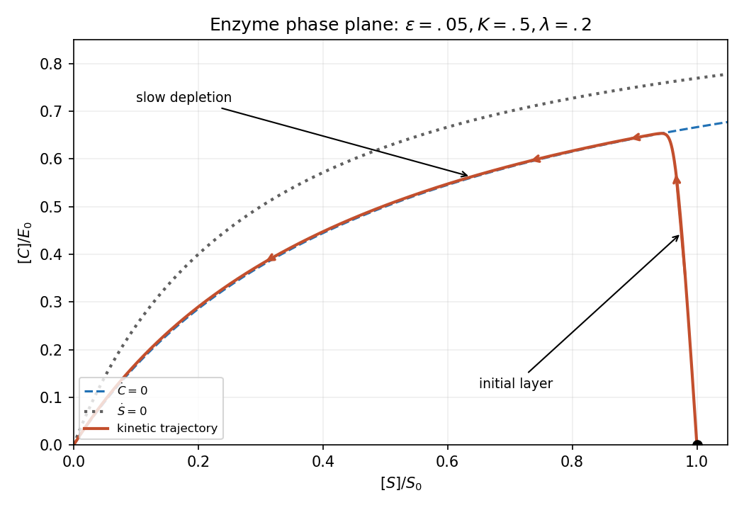
Enzyme kinetics in scaled concentration coordinates: rapid complex buildup followed by slow substrate depletion
. Details. 
The official Oxford course archive advertises an answer for this entire question. Its introductory ask and all seven leaves are covered externally and are not re-solved here.
The decreasing production term represents negative feedback: low red-cell abundance stimulates production, whereas high abundance suppresses it. The linear loss term models removal at constant per-cell rate. SetThen , with . On the physical half-line , decreases from one to zero while increases from zero to infinity. Their unique intersection is the steady state. Its linear derivative is , so it is asymptotically stable.
For small , the intersection lies at large , where ; for large it lies at small , where . HenceImplicit differentiation of gives . The plot joins these two decreasing asymptotic regimes.
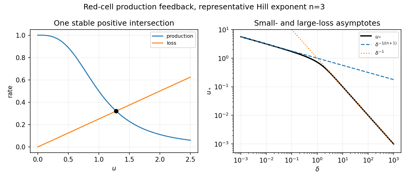
Negative production feedback gives one stable red-cell equilibrium and two limiting concentration scalings
. Details. 
The delay represents the time between feedback sensing and the appearance of newly produced mature cells. In dimensionless time it is , so the equation becomesIt requires a nonnegative initial history on , not just one initial value. Its constant equilibrium is unchanged. Put . A small perturbation obeys , whose characteristic equation isThere is no real root with , because all three terms would have positive sum; zero is never a root either. Starting from the stable zero-delay case, loss of linear stability can therefore occur only when a complex conjugate pair crosses the imaginary axis at a nonzero frequency, the linear signature of a Hopf bifurcation.
For completeness, substituting gives and . Such a crossing requires , withThe first crossing is transversal: . If , the magnitude relation rules out roots in the closed right half-plane for every delay. A nondegenerate nonlinear Hopf conclusion additionally uses the usual bifurcation hypotheses. This is delayed negative feedback in red-cell production.
Resting cells enter proliferation at rate . A proliferating cell takes a fixed cycle time to divide and survives that cycle with probability under a constant death hazard . Thus exit from the proliferating compartment at time is , and it returns twice as many daughter cells to the resting population. Resting-cell loss at rate is separate.
More explicitly, the number currently in the proliferating stage isfor a consistent initial history. Differentiation gives the stated equation. Counting resting-cell entry, loss and daughter-cell return gives its equation. Negative feedback in suppresses recruitment when the resting population is high; its Hill exponent gives a steep response around the concentration scale .
Set and defineThen , so the resting-cell equation becomes exactlyThe nonzero steady state solves , or for positive . The latter right side decreases strictly from to zero. Thus when there is exactly one positive equilibrium,Zero is also an equilibrium; negative populations are outside the biological domain. The same result is visible by intersecting the line with the hump-shaped .
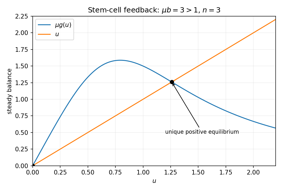
Resting-cell recruitment feedback has one positive equilibrium when the small-population reproduction factor exceeds one
. Details. 
Put . Linearization and a mode giveHere is the coefficient called in the source's characteristic equation; it is not the proliferating-cell death hazard. Any characteristic root with positive real part makes the equilibrium linearly unstable. A nonzero imaginary crossing satisfies and ; these are its Hopf conditions, subject to nondegeneracy.
On slow time , the unit delay becomes . Taylor expansion gives . Dividing the equation by therefore yieldsThis approximation requires slow smooth variation and a denominator bounded away from zero; a vanishing denominator marks failure of this slow reduction. On the fast time , omit only the explicit order- terms, retaining the finite delay:Replacing the delayed argument by the present value on that fast scale would incorrectly erase the dynamics. These are the slow and fast limits of a delayed stem-cell model.
Articles by others on the same topic
There are currently no matching articles.