Write for the homogeneous cubic correction and for the nilpotent linear part. The chain rule gives the transformed cubic vector field as . Thus the cubic coefficients in the first equation arewhile those in the second equation areConsequently one explicit near-identity transformation isThe transformed equations have no cubic correction in , and only survive in . The cubic coefficients areThis is the cubic elimination at a nilpotent double-zero point; the extra is the nilpotent cubic damping invariant contribution from the first equation. Higher-order terms generated by the substitution are outside the cubic truncation.
The linearization of this reduction of the FitzHugh-Nagumo model at its trivial equilibrium point isA double zero eigenvalue requires both the constant and linear coefficients to vanish. Hence the codimension-two point isThere the polynomial is . The kernel of a linear map of is one-dimensional, so its zero eigenvalue has a nontrivial size-two block in Jordan normal form. This is a reflection-symmetric double-zero point of Bogdanov–Takens bifurcation type, with one stable direction; the nonlinear coefficients are computed below rather than assumed.
A simple zero eigenvalue occurs on , except at . The odd symmetry of the vector field gives a pitchfork bifurcation. Near this curve the critical eigenvalue isFor the other two eigenvalues are stable: this is a supercritical pitchfork bifurcation as decreases through . For it is a subcritical pitchfork bifurcation in the center direction, with an already unstable transverse direction.
For a Hopf bifurcation, factor the characteristic polynomial as . Comparing coefficients givesThus the trivial branch has the local bifurcation curvesThe second curve is a Hopf bifurcation with a stable third eigenvalue. The Routh-Hurwitz stability criterion gives the stable trivial region , . Its Hopf bifurcation is subcritical. To check the sign, normalize the critical right eigenvector by and putThe second component of the normalized left projection is . There is no quadratic term at the origin, and the cubic derivative in the second component is . The cubic Hopf coefficient is therefore . A small repelling periodic orbit lies on the stable-origin side. The diagram also includes the nonzero-branch information derived next.
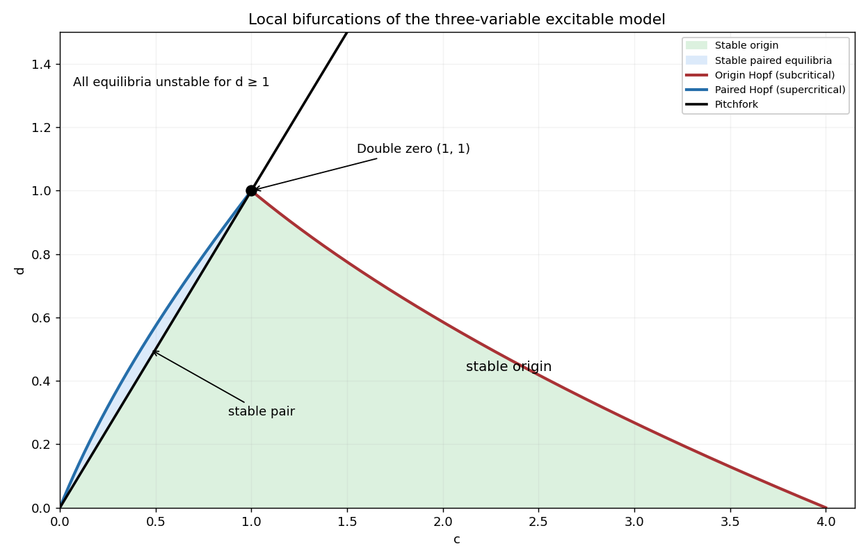
The nonzero equilibrium points are paired by reflection:At either equilibrium point, the derivative of the second equation with respect to is . The characteristic polynomial becomesIts constant term is nonzero away from the pitchfork bifurcation, so there is no further steady local bifurcation. At a Hopf bifurcation the condition givesIndeed and require ; within this range is equivalent to . The apparent singularity at does not hide another solution of the coefficient equation. The Routh-Hurwitz stability criterion shows that both equilibrium points are stable for , , and unstable for . For , , so no nonzero equilibrium point is stable.
Their Hopf bifurcations are supercritical. Here is a coefficient check that includes the effect of the quadratic term around . Let , and normalize as before. The inverse-linearization term has . AlsoThe resonant cubic Hopf coefficient isIn this simplification . Thus stable small periodic orbits appear around each nonzero equilibrium point on the side. This classifies the local branches; the sketch does not infer uncomputed distant global bifurcations.
The specified coordinate change gives the exact equationsAt linear order on the center manifold. More precisely the stable coordinate obeys at linear order, while , . Thus relaxes towards its center-manifold value and can be eliminated by center manifold reduction or a properly ordered adiabatic elimination.
Write , where is homogeneous of degree . At degree two the graph invariance equation is . On homogeneous quadratic polynomials the operator is nilpotent, so adding makes it invertible. Hence . Equivalently, the odd vector field permits a symmetry-compatible odd graph: odd symmetry removes even center-manifold jets. No quadratic forcing is present for adiabatic elimination either. However, setting alone is insufficient at cubic order, because the evolving graph has a nonzero derivative.
To include the stable-variable lag in nilpotent center-manifold reduction, let . Invariance of the center manifold requiresFor the homogeneous polynomial , comparison of coefficients successively givesOnly is needed for the requested cubic normal form. The reduced first equation has ; the reduced second equation, obtained by replacing with in its cubic term, has and . Therefore the cubic elimination at a nilpotent double-zero point yieldsIn particular, ignoring the lag and imposing exactly would incorrectly give . The full cubic graph above provides a direct substitution check.
Use the Galerkin method, rather than pointwise equality: products generate harmonics outside the retained five-dimensional space. Put , , and denote the five prefactors byThe retained streamfunction is , the retained temperature perturbation is , and the retained magnetic-flux perturbation is . These satisfy all the stated boundary conditions. Let , the streamfunction advection bracket. Orthogonality of the sine and cosine modes gives the following coefficients of the retained harmonics:For example the contribution to the temperature bracket is . The magnetic bracket follows by writing : and . These identities exhibit both the retained terms and discarded harmonics.
Before rescaling time, the projected coefficient equations areSubstitute the prefactors and divide time derivatives by . With , and , the resulting five-mode vertical-field magnetoconvection equations areHere primes denote differentiation in . The factor is , which checks the magnetic nonlinear sign. There is a terminology qualification in the source: on this thermal diffusion time scale, its is the magnetic-to-thermal diffusivity ratio . The conventional magnetic Prandtl number is , where is the Prandtl number. The displayed equations and subsequent calculation use the source's unchanged.
At conduction, and have stable eigenvalues and . The remaining linearization on isIts characteristic polynomial is , whereConsequently the steady threshold is . The symmetry , with unchanged, gives a generic pitchfork bifurcation, whose forward or backward direction is determined below. At threshold the other two critical-block eigenvalues satisfy , where . They are stable if ; if there is already one unstable transverse direction. Degenerate zero cubic slope requires higher-order analysis and is not a generic pitchfork.
At a Hopf bifurcation, , . Solving the coefficient equation givesFor physical the oscillatory threshold therefore exists exactly when and . The conduction double-zero criterion for five-mode magnetoconvection givesAt this Bogdanov–Takens bifurcation, the polynomial is and the zero eigenspace is one-dimensional. For conduction first loses stability at the steady threshold; for it first loses stability at . For no positive- double-zero or oscillatory threshold exists. These conclusions also follow from the Routh-Hurwitz stability criterion, and . The Hopf bifurcation is transversal since ; its nonlinear criticality is not required by this linear onset calculation.
On the nonzero stationary branch of five-mode magnetoconvection, put and . The temperature equations first give and . The magnetic equations then giveDivide the steady first equation by and substitute these expressions. The exact branch isExpanding at givesNear the required amplitude restriction ensures . For , , so the paired equilibrium points emerge in the forward direction . For fixed and small , the pitchfork reversal near geometric ratio two in magnetoconvection occurs atThis follows by expanding the exact zero-slope equation . Above this value the branch initially runs backwards into ; at there is no reversal. This is a degenerate pitchfork bifurcation at , not a conclusion that every emerging state is stable. If , the center-direction cubic term has the opposite sign to : the forward branch is locally attracting and the backward branch repelling. If , an unstable transverse mode remains.
For the nearby geometry, the next coefficient is , which is negative near the reversal. Thus a small positive produces a nearby maximum of at ; this fold approaches the pitchfork as . Once the small-amplitude branch is backward. The exact formula eventually grows like , so a backward branch must turn at a finite amplitude, potentially outside the small-amplitude expansion.
The equilibrium points satisfy , . For there are none. For set . The Jacobian matrix isThe positive equilibrium point is always a saddle equilibrium. At the determinant is , so it is stable for and unstable for . The discriminant distinguishes a node from a focus; its zero does not destroy hyperbolicity and is not another local bifurcation curve.
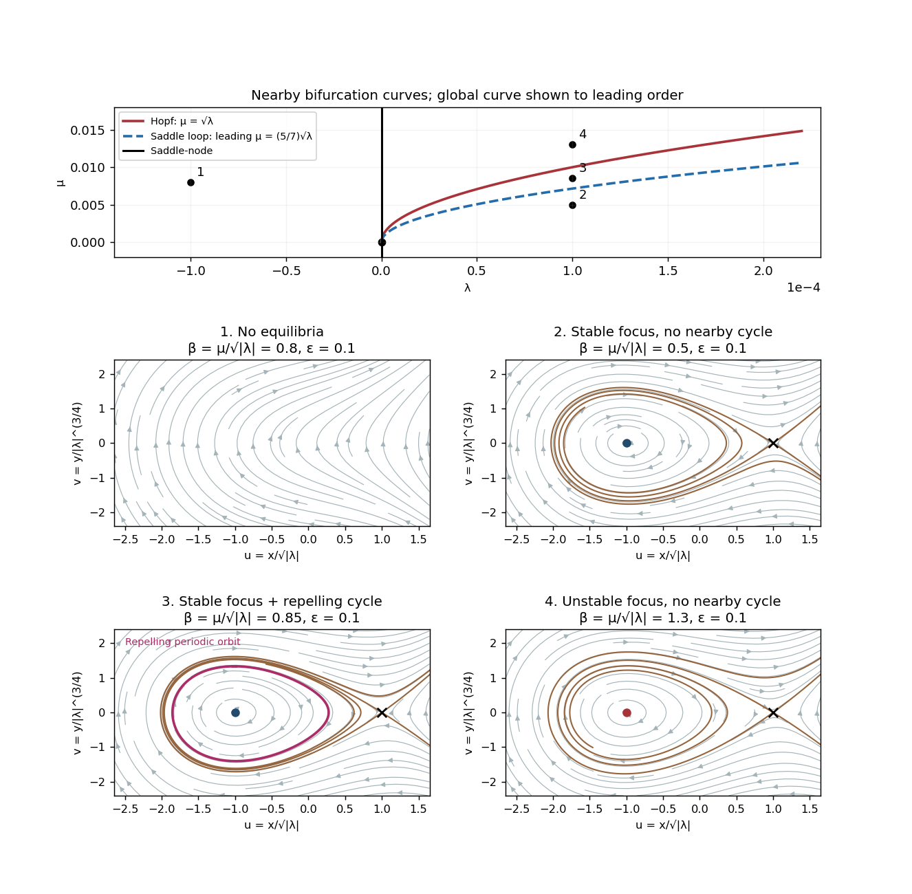
The local bifurcation curves areAt the linearization has a double zero eigenvalue and is nilpotent, giving a Bogdanov–Takens bifurcation. For on , solving the local center manifold gives , displaying the saddle-node bifurcation. For the nonsaddle branch born at positive is attracting; for it is repelling. On the Hopf curve the angular frequency is . The permitted subcritical Hopf bifurcation creates a repelling periodic orbit on the stable-focus side .
A local analysis alone does not say how far that periodic orbit extends. The global calculation below supplies the additional division of the stable-focus region. The complete nearby phase portraits and the leading global curve are shown together here. The flow has no closed periodic orbit, since a closed orbit would have index one and hence enclose an equilibrium point.


Substitution of the weighted scaling and givesThe derivative of the candidate Hamiltonian isThus is a conserved quantity at . For put . The conservative equilibrium point is a center with , and is a saddle equilibrium with saddle-loop energyThe closed component of a level between these energies surrounds the center. At ,is the homoclinic orbit, with left turning point . The upper branch is traversed to the right and the lower branch to the left. Levels above the barrier have escaping trajectories; the saddle level also has unbounded branches to the right. For the two critical points coalesce; for the potential is monotone and there is no center or saddle loop.
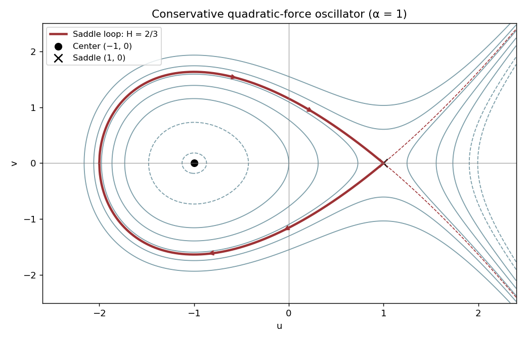
Hamiltonian level curves and the conservative saddle loop for alpha equal to one
. Details. 
Along a perturbed saddle loop the incoming and outgoing endpoints have the same Hamiltonian value. Integrating and evaluating the leading integral on the conservative homoclinic orbit givesOn the upper half of the loop and . The lower half makes an equal contribution, soThese homoclinic integrals for a quadratic-force oscillator give the simple first-order splitting zero , since . The Melnikov energy-balance method therefore yields the leading global bifurcation curveThis is an asymptotic curve near the double-zero point, not an exact finite-parameter identity. More precisely, time reversal preserves the loop condition. The smooth curve selected by its simple splitting zero is even in , giving and hence for fixed scaled .
Between the saddle-loop curve and , a stable focus is surrounded by the repelling periodic orbit created at the subcritical Hopf bifurcation. As decreases, this orbit grows until it reaches the saddle. Below the saddle-loop curve there is a stable focus and a saddle, but no nearby cycle. Above the Hopf curve there is an unstable focus and a saddle, with no nearby cycle. At the global curve the saddle separatrices form the repelling loop. Under the stipulated absence of further bifurcations, these are the distinct nearby regions in the earlier sketch; no extra remote phase structure is being inferred from the leading-order calculation.
At the saddle equilibrium , put . The two eigenvalues and saddle index areOn the nearby saddle-loop curve, . Therefore , with the more explicit expansionThe positive saddle quantity makes the loop repelling. In a transverse section its leading return map has the form ; its derivative grows without bound as . This is the mechanism by which a positive saddle quantity makes a nearby saddle loop repelling. It agrees with the repelling periodic orbit coming from the subcritical Hopf bifurcation, rather than predicting an attracting cycle at the collision.
Articles by others on the same topic
There are currently no matching articles.