An affine connection on the tangent bundle of a smooth manifold assigns a vector field to two vector fields, is -bilinear, and satisfiesThus its first slot is tensorial and its second obeys the Leibniz rule. Its action on covectors is defined by differentiating the pairing, and this extends it to tensor fields. A torsion-free connection has .
Assume that is a smooth nondegenerate metric tensor. Metric compatibility and a vanishing torsion tensor imply the Koszul formula,The right-hand side is determined by and the Lie bracket of vector fields. Nondegeneracy determines uniquely; conversely this formula defines an affine connection with both required properties, proving existence as well as uniqueness. In a coordinate frame the brackets vanish. Combining the three differentiated metric tensor identities givesThis is the Levi-Civita connection. Positive definiteness is unnecessary: the argument also works for a pseudo-Riemannian metric.
For the other affine connection define . The derivative of cancels between the two Leibniz rules, so is -linear in both slots. The difference of affine connections is a tensor: here is a section of with components . Both affine connections are torsion-free, so .
Agreement of geodesics means agreement of their unparametrized curves; different affine parameters are allowed. For every nonzero tangent vector , existence of a geodesic with that initial velocity implies that is parallel to . The symmetric bilinear diagonal-parallel lemma now determines . Choose a basis and write . Applying the parallelism condition to and givesWith , bilinearity yieldsThis is projective equivalence of affine connections. It also covers dimension one. For two Levi-Civita connections, the projective covector from metric volume densities gives the explicit answerIndeed . The determinant ratio is a scalar, so this expression is a genuine covector, although either determinant alone is coordinate-dependent. This determinant expression requires nondegeneracy of ; the difference-tensor and earlier trace formula require only the two torsion-free affine connections.
Conversely, the displayed tensor gives along an affinely parametrized -geodesic. Choosing a new parameter satisfying removes that tangential acceleration. This geodesic reparametrization under projective equivalence proves sufficiency. If agreement were required with the very same affine parameter, polarization would instead force and .
Use , background Minkowski spacetime metric tensor , and with small metric perturbation. All indices and derivatives in this linear approximation use . The linearized inverse metric is , and the linearized Levi-Civita connection isDefine the trace-reversed metric perturbation , with .
An infinitesimal coordinate change gives the linearized coordinate gauge transformationThe metric perturbation therefore has redundant components. The gauge invariance of the linearized Riemann tensor follows because its change contains third derivatives of cancelling by commutation of partial derivatives. Conversely, flat linearized metric perturbations are locally pure gauge on a contractible patch. Thus linearized curvature, rather than a particular coordinate value of , detects the physical disturbance. Gauge freedom can also be restricted by global topology or boundary conditions.
Keeping the paper's curvature sign convention, its linearized Ricci tensor and scalar areThese are the negatives of the alternative frequently used curvature convention. Put . The Linearized Einstein equations in vacuum areUnder a gauge change , so solving imposes the Lorenz gauge in linearized gravity. The field equations then become . The remaining residual gauge symmetry of linearized gravity has ; Lorenz gauge does not exhaust the coordinate freedom.
A Fourier mode obeys and . Hence the plane gravitational waves in linearized gravity propagate on the background light cones. Four transversality conditions and four residual gauge amplitudes leave physical degrees of freedom. The explicit plane-wave reduction to transverse-traceless gauge can set , spatial trace zero and . For a wave in the direction, write its physical spatial strain as , so the spatial metric tensor is :There are two gravitational wave polarizations, plus polarization and cross polarization. Rotating transverse axes through rotates their amplitude pair through . Nonconstant profiles with nonzero second derivative have nonzero linearized Riemann curvature tensor and cannot be removed as pure gauge.
The TT coordinate separation and measured separation distinction explains a detector's response. Freely falling particles initially at rest can keep fixed TT coordinates, since , while their proper separation changes. For a short arm along a unit vector ,This is the tidal response described by geodesic deviation; coordinate motion by itself is not the measured signal.
Finally, gravitational-wave energy is second order in the perturbation, so it is absent from a first-order vacuum equation. In a short-wavelength averaging regime the averaged stress-energy of transverse gravitational waves isFor a plane wave its energy flux is . The averaging scale and weak-field assumptions matter: this does not assign a coordinate-independent local gravitational energy density to an arbitrary first-order perturbation.
The Brans-Dicke theory couples a scalar field to the Ricci scalar. Assume , constant , matter independent of , and variations of compact support so boundary terms may be discarded. Use the paper's curvature sign convention and signature . Set and . Define the stress-energy tensor consistently byThis convention fixes the sign of the matter term.
Vary with respect to . The variation of metric volume density contributes times each scalar Lagrangian, while . Applying the Palatini identity followed by two rounds of integration by parts gives the metric variation of a scalar-curvature coupling,The differentiated terms remain because the curvature multiplier is not constant. Varying the kinetic term at fixed givesCombining these terms with the matter variation, the Euler-Lagrange equation isRaising both free indices reproduces the contravariant form, because .
The independent scalar variation givesor . The trace of the metric tensor equation in four dimensions isMultiplying the scalar equation by eliminates the same combination . Thus the scalar equation of Brans-Dicke theory isAt the degenerate coupling of Brans-Dicke theory, , the combined equations impose instead; division by is unavailable. If matter depended directly on , its scalar variation would add a source and the displayed scalar equation would change.
The following lettered sections justify the supplied variation identities; they are supporting identities in the PDF, rather than three independent field-equation problems.
Differentiate while holding the coordinate system fixed. The variation of inverse metric obeysMultiplication by the inverse metric tensor givesThis is the matrix inverse derivative written with tensor indices. A variation of the metric tensor is symmetric, so the right-hand side is symmetric in .
Write . The Jacobi formula gives . Since a Lorentzian metric of signature has negative determinant,The variation of metric volume density therefore has the opposite sign when expressed using the inverse metric tensor: . This follows immediately from the variation of inverse metric and explains the volume term in the field-equation derivation.
Although connection coefficients are not tensor components, their variation is tensorial: the difference of affine connections is a tensor. Varying the Levi-Civita connection at fixed coordinates givesIn the paper's curvature sign convention, varying the derivative and quadratic-connection terms and grouping them into covariant derivatives gives the Palatini identityOne may verify the grouping in normal coordinates at a point, where the affine connection vanishes and the expression is just the difference of two partial derivatives; both sides are tensors, so it holds in every coordinate frame. Reversing the definition of the Riemann curvature tensor reverses this identity's right-hand side.
For completeness, put and . The contracted variation uses and . After two integrations by parts,up to the discarded boundary term. Substituting gives the differentiated-scalar terms in the metric variation of a scalar-curvature coupling.
The local metric tensors do not determine the global coordinate identifications. The usual complete two-dimensional de Sitter spacetime is the hyperboloid in ambient signature , withPulling back the ambient metric tensor gives , withUnwrapping gives the universal cover of two-dimensional de Sitter spacetime instead. The usual embedded two-dimensional anti-de Sitter spacetime has in signature andHere and is initially periodic modulo . The time circles are closed timelike curves. Its physically standard universal cover removes that identification:The two signs of describe two spatial ends; imposing would retain only half of this complete model.
Both spacetimes have constant curvature and are geodesically complete. In the paper's convention their Ricci scalars are respectively and . Their embeddings show that geodesics are intersections with planes through the ambient origin. They nevertheless have very different causal structures.
For the geodesics of two-dimensional de Sitter spacetime, use an affine parameter , normalization and conserved momentum . ThenTimelike geodesics extend to both infinite proper times; is a simple example. Null geodesics obey , so their affine parameter is also infinite at either temporal end. Spacelike geodesics have , obey and are closed curves on the embedded cylinder; is its simplest spacelike geodesic circle. Unwrapping the spatial circle removes closure but not completeness.
For the geodesics of two-dimensional anti-de Sitter spacetime, the timelike Killing vector gives . The normalization is , henceChoose a future-directed timelike geodesic, so andFor , it oscillates radially with proper period ; gives the central geodesic . In both cases, global time advances by over a proper time interval . The curve is closed on the original hyperboloid, while its lift on the universal cover is nonclosed and future-directed. Null geodesics have and reach either spatial end only at infinite affine parameter. Spacelike geodesics satisfy and also have infinite proper length toward either end. Thus the finite coordinate time discussed below does not imply physical geodesic incompleteness.
The conformal cylinder of two-dimensional de Sitter spacetime follows by setting :Its past and future conformal boundaries are spacelike circles. Null geodesics have and can travel only a finite angular distance over the entire infinite proper-time history. For the complete observer , an event can send a signal to that observer precisely when its shortest angular distance is less than . The observer horizons in two-dimensional de Sitter spacetime are therefore the null curves ; its past signal horizon has . These are observer horizons, without curvature singularities. Their intersection bounds a static patch with metric tensorThe horizons at are regular Killing horizons beyond which this static chart fails, while the global coordinates remain smooth.
For the conformal strip of two-dimensional anti-de Sitter spacetime, set . On its universal cover,The two conformal boundaries are timelike. A null ray from the center approaches a boundary after coordinate time , though its affine parameter diverges. Every interior event can signal to the complete central static observer in finite global time, so that observer has no event horizon. A Poincaré horizon concerns a restricted coordinate patch, and accelerated observers can have different causal horizons.
Finally, the global de Sitter cylinder and its spatial cover are globally hyperbolic: constant-time slices are Cauchy hypersurfaces. The anti-de Sitter universal cover is not globally hyperbolic, because timelike infinity admits incoming signals within finite global time. A field's evolution therefore requires boundary conditions at its two conformal boundaries in addition to initial data. The opposite placement of the conformal boundaries explains why de Sitter observers have cosmological horizons despite global hyperbolicity, while the central anti-de Sitter observer has no event horizon despite the failure of global hyperbolicity.
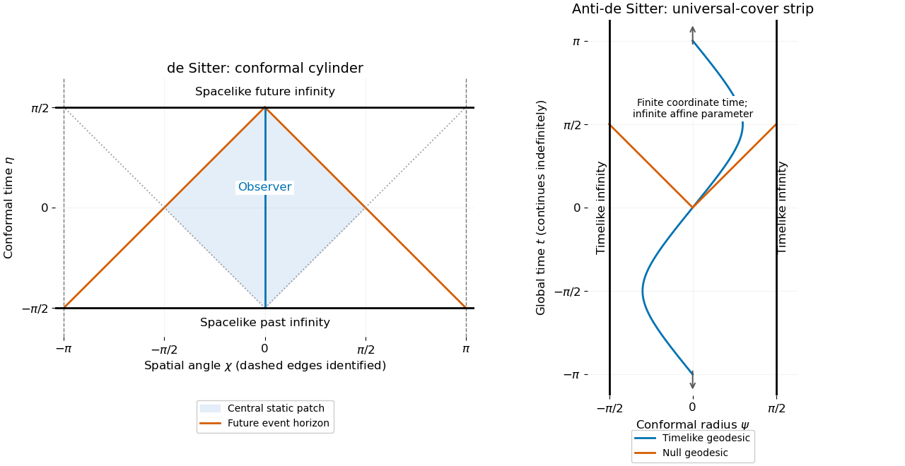
Conformal cylinder and observer horizons of de Sitter spacetime compared with the timelike boundaries of the anti-de Sitter universal cover
. Details. 
Articles by others on the same topic
There are currently no matching articles.