Write the expected value as and assume the relevant covariance matrix is invertible. Remove the linear predictor from the first block by definingA linear image of a multivariate normal vector is again multivariate normal. Direct covariance calculation givesThus and are independent: uncorrelated jointly Gaussian variables are independent. Expanding the covariance matrix of , using , givesConditioning on translates by the fixed vector and leaves its covariance matrix unchanged. Consequently the conditional multivariate normal distribution isThe conditional covariance is the Schur complement and does not depend on .
Put , the precision matrix, with scalar and containing all remaining coordinates. Holding in the multivariate normal density, the terms involving in its exponent areCompleting the square gives a normal distribution with mean andEquivalently, the block matrix inverse identity gives . The Gaussian conditional variance from precision is a reciprocal diagonal entry of the precision matrix, rather than the marginal variance .
Write and . Apply the Schur complement covariance to the first two coordinates, conditioning on the third. The conditional covariance and conditional variances areDivide the conditional covariance by the product of the conditional standard deviations. The conditional correlation is thereforeThis is the partial correlation after removing the linear effect of . For a nonsingular multivariate normal distribution, both residual variances are positive and the answer is independent of . If a residual variance vanishes, the requested correlation coefficient is undefined, even though the residual covariance formula remains valid.
Use the usual sample mean and the divisor- sample covariance matrix,The residual sum is zero, so expanding givesMultiplying the independent multivariate normal densities and taking logarithms yields the log-likelihoodHere is the determinant and denotes the trace. The maximum-likelihood estimators areIf instead denotes the divisor- sample covariance matrix, replace by and then . These formulas describe a nonsingular maximum-likelihood estimator when the empirical scatter is positive-definite; if it is singular, there is no maximizer over positive-definite covariance matrices.
Let , and . Define the within-group and between-group scatter matrices byThe within-group and between-group scatter decomposition gives total scatter : in each group the residuals about sum to zero, so all cross terms vanish. Under unrestricted group means, the maximum-likelihood estimators are and . Under the common-mean null hypothesis, they are and .
For either fitted scatter matrix , substitution into the log-likelihood givessince . Thus the maximized likelihood ratio isA generalized likelihood-ratio test rejects for small , equivalentlyThe cutoff is chosen for the desired significance level. The determinant ratio itself is the Wilks lambda statistic. The derivation assumes is positive-definite, which for continuous normal samples requires enough within-group degrees of freedom, ; singular does not support this ordinary determinant-based test without a modified model.
The within-group and between-group scatter decomposition separates noise from group separation: measures variation about each group sample mean, and measures separation of those means about the overall sample mean. In linear discriminant analysis, seek a projection maximizing between-group relative to within-group variation,Normalize by ; a Lagrange multiplier calculation gives the generalized eigenvalue problem . The leading canonical discriminant directions have the largest eigenvalues, and subsequent directions are orthogonal in the inner product. There are at most nonzero separating directions. Projecting observations onto these directions gives a low-dimensional display of group separation.
For classification, estimate the common covariance matrix by and use the linear discriminant analysis scoreswhere are class prior probabilities. Assign to the largest score. The same within-group scatter sets the noise scale, while between-group scatter selects the directions in which the group means separate most strongly.
The first command reads a rectangular data file into
a; header=T treats the first line as variable names. There are twelve observations, identified by student names, and nine binary attributes. A one records presence of an attribute and a zero records absence. This is a description of the encoding, not a claim that every presence is equally important for a scientific application.dist(a, metric="binary") compares rows using Jaccard distance. If counts shared presences and count mismatched presences, thenJoint absences do not enter the denominator, unlike the simple matching coefficient or normalized Hamming distance. dist2full(d) expands the stored pairwise distances into a symmetric dissimilarity matrix; round(...,2) changes only its displayed precision. The clustering command still receives the original unrounded distances.For example, Tom and Martin have six shared presences and only one mismatch, giving . Taeko and Luitgard have three shared presences and four mismatches, giving . LingChen and Mohammad share only the meat attribute and differ on four others, giving . The diagonal is zero, and the entries are symmetric because exchanging the two observations exchanges and .
hclust(d, method="compact") constructs an agglomerative hierarchical clustering object by complete-linkage clustering. Its distance between two current groups isStart with singleton groups, merge a pair with smallest intergroup distance, update these maximum cross-pair distances, and repeat until one group remains. The object stores the merge structure, merge heights and a leaf order suitable for a dendrogram; assigning it to h does not itself display a graph. The historical S-Plus help identifies compact with complete linkage and describes the plotting object.The first merge is Tom with Martin at . At the next height , either LinYee with HuiChin or HuiChin with Meg may merge: the distances are tied. The following dendrogram shows one valid resolution, using original row order to resolve ties. In this tree, LinYee joins HuiChin at , Pio joins Meg at , and Nicolas joins Tom–Martin at . The latter height is , illustrating the complete-linkage update.
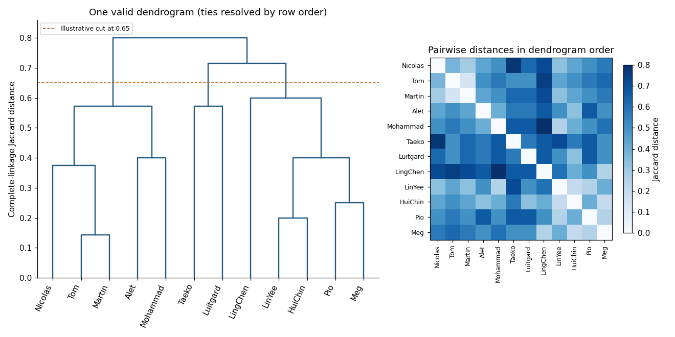
Complete-linkage dendrogram and Jaccard-distance heatmap for the binary student profiles, with one valid tie convention
. Details. 
For the displayed tree, a cut at height gives three groups: Taeko–Luitgard; Alet–Tom–Martin–Nicolas–Mohammad; and LinYee–Pio–LingChen–HuiChin–Meg. The last two merges occur at and . The hierarchy is a description under the chosen binary distance and linkage rule; it neither supplies an intrinsically correct number of groups nor guarantees a unique tree in the presence of ties. Changing the treatment of joint absences, or the weighting of attributes, can change that description.
princomp(): principal component analysis. Supply observations in rows and numeric variables in columns. After centering, let denote the resulting matrix and its sample covariance matrix, with an explicitly stated normalization. WriteThe first direction maximizes the Rayleigh quotient over unit vectors; successive directions maximize it subject to orthogonality to the earlier directions. The principal component scores are , with variances and zero pairwise sample covariance. Zero covariance alone does not imply independence. Each principal component loading describes a direction in variable space; its sign is arbitrary, and repeated eigenvalues leave the basis inside the corresponding eigenspace arbitrary.The function returns principal component loadings, component standard deviations
sdev and, when requested, principal component scores. By default it uses a covariance matrix; cor=T instead performs principal component analysis on a correlation matrix, standardizing nonconstant variables to variance one. This choice matters when variables have different measurement units. These interface details are documented in the S-Plus help for princomp.A scree plot shows the ordered eigenvalues; a plot of the first two principal component scores can reveal groups, unusual observations or a dominant gradient. The first components explain of the total variance. Reconstructing each centered observation by its orthogonal projection onto these directions minimizes average squared reconstruction error among -dimensional linear subspaces. Thus PCA gives an optimal linear compression for squared reconstruction error, with scaling and the retained dimension chosen explicitly. It is an unsupervised learning method, rather than a classification rule fitted to supplied labels.
tree(): classification trees and regression trees. A call such as tree(response ~ predictors, data=dat) fits a recursive partitioning model. At a current node, test numerical predictors against candidate thresholds, or divide the levels of a categorical predictor into two sets. Select a split that most improves the fitting criterion, then repeat within its children. Numerical splits give axis-aligned regions. A categorical response produces a classification tree; a numeric response produces a regression tree, as specified in the S-Plus tree documentation.For a regression tree, the constant prediction in a terminal region is its sample mean, minimizing the sum of squared residuals there. For a classification tree, estimate class probabilities by the observed proportions in a leaf and predict a most probable class under equal misclassification costs. The classification-tree deviance of a node iswith ; splitting maximizes the decrease from parent to children. This fitting criterion differs from the number of wrong classifications. The middle sketches show the same three-region partition as a binary tree: first split on variable one, then split the right-hand branch on variable two.
Growing to small leaves can overfit. Use cost-complexity tree pruning, balancing fitted loss against leaf count,and select complexity by cross-validation. Plotting the fitted tree and annotating nodes displays the rules; prediction routes each new observation through the fitted splits. A tree gives an interpretable, piecewise-constant prediction rule; training fit alone does not measure prediction accuracy.
The
rpart() alternative. This also fits classification and regression trees by recursive partitioning, with squared-error splitting for ordinary numeric responses and, by default for classification, Gini impurity . Classification settings can instead use information-based splitting and specify prior probabilities and a loss matrix. It supports surrogate splits to approximate a node's primary left/right assignment when the primary predictor is missing. Its complexity-parameter path and cross-validated errors support cost-complexity tree pruning; for example, select a complexity parameter and apply prune(fit, cp=...). The maintainer's rpart documentation describes the criteria and the distinction in handling surrogate predictors. The partition and tree sketches apply to either implementation; the fitted tree need not be the same because splitting criteria and controls can differ.cmdscale(): classical multidimensional scaling. Its input is a dissimilarity matrix or stored distance object. It outputs coordinates for the observations in a chosen dimension, usually two for visualization. Let contain the squared entries of , and putFor centered Euclidean coordinates , the distance identity gives : multiplying by removes the row and column norm terms. Diagonalize this Gram matrix and retain its largest positive eigenvalues. The coordinates areThus classical scaling exactly recovers Euclidean distances when all positive eigenvalues are retained. Reducing dimension approximates the centered Gram matrix; it does not in general minimize squared discrepancies in the original distances. Negative eigenvalues identify a failure of the Euclidean distance matrix criterion, so their size matters when interpreting a display. The historical S-Plus cmdscale help describes the dimension argument, eigenvalue output and optional additive adjustment to dissimilarities.Plot the two coordinate columns on equally scaled axes and label observations. Nearby plotted points suggest small dissimilarities only insofar as the dimension reduction fits the input well. The bottom sketches give an exact Euclidean example: a configuration and its independently recovered two-dimensional coordinates have identical pairwise distances, despite different coordinate axes. Classical scaling converts distances into geometry; translations, rotations and reflections do not change the represented distances. For Euclidean distances between observations, its coordinates agree with the corresponding principal component scores up to these harmless choices of axes.
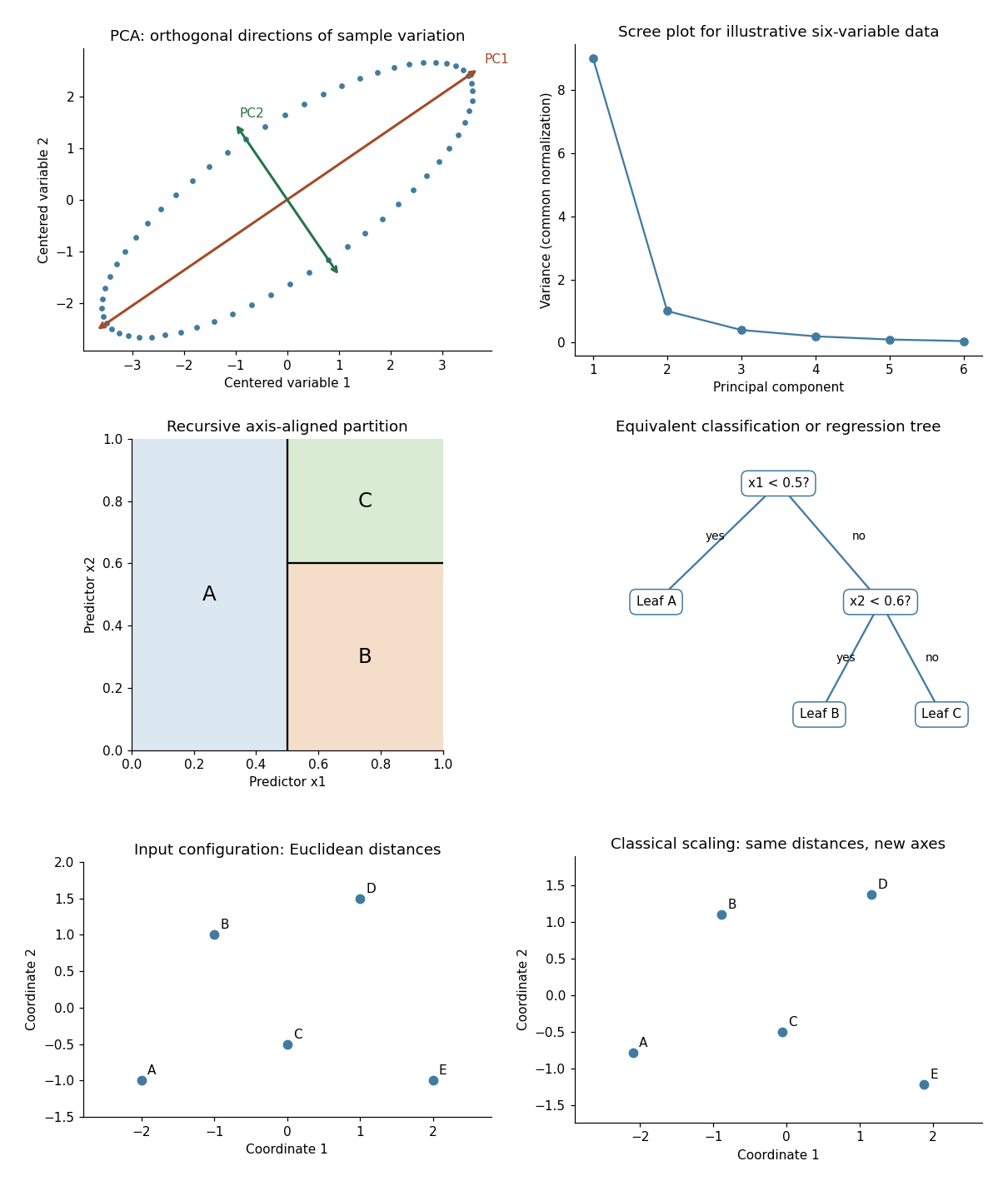
Illustrative PCA directions and scree plot, equivalent recursive partition and tree, and exact classical-scaling recovery of Euclidean distances
. Details. 
Under equal costs for either wrong assignment, the Bayes classifier chooses the class of greatest posterior probability. With positive prior probabilities, it assigns class one when ; ties can be resolved arbitrarily. For the two multivariate normal densities with common positive-definite covariance matrix , their normalizing factors cancel. The log posterior odds areTherefore the Gaussian Bayes classifier has the required linear form, withA larger prior probability for class one decreases , expanding its decision region. The prior-dependent Gaussian discriminant boundary is the hyperplane .
For equal prior probabilities, . The projected score is normal under either class because it is a linear image of a multivariate normal vector, and its variance isMoreover , so the midpoint threshold lies from either projected mean. HenceStandardizing the two normal distributions, with the standard normal distribution function, givesThus the equal-covariance Gaussian classification error is . The Mahalanobis distance between the class means is their separation in units of within-class noise. It yields as and as . The stipulated means the two class means are distinct.
Articles by others on the same topic
There are currently no matching articles.