Assume a steady, incompressible, inviscid flow with a nearly uniform velocity across each water section. The channel varies slowly enough for vertical accelerations to be negligible, pressure to be hydrostatic and the water surface to be nearly horizontal across the width. Atmospheric pressure is uniform; neglect surface tension, wall friction and energy losses. The hydraulic equations apply away from jumps and short nonhydrostatic regions.
The Euler equation for horizontal momentum, with hydrostatic pressure, givesIntegrating gives a constant Bernoulli equation head . Conservation of mass gives the constant volume discharge . Thus the shallow-water specific energy, measured above the local bed, isDefine the Froude number by for the positive flow direction. ThenAt fixed discharge and width, energy tends to infinity at both zero and infinite depth. It has a unique minimum atIndeed . Above the minimum there are two depth branches: the shallower one is supercritical flow and the deeper one is subcritical flow.
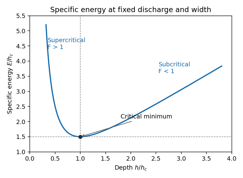
Specific-energy minimum and the subcritical and supercritical depth branches
. Details. The local long-wave propagation speeds from the shallow water equations are . In subcritical positive flow, one wave family travels upstream and one downstream. In supercritical flow both travel downstream. At critical flow the upstream-directed speed is zero, so the flow can provide hydraulic control separating upstream adjustment from downstream conditions. This statement concerns long waves in the slowly varying hydraulic approximation, rather than all short-wave disturbances.
For a smooth positive discharge on the flat bed, differentiate the constant specific energy. With ,At a regular critical point, and , so . Since is constant, this requires . The given width has , proving that a regular hydraulic control can occur only at .
The throat is the unique width minimum and hence the maximum of the critical-energy envelopeA steady positive-depth flow must have its conserved energy at least as large as every local minimum energy. To be controlled smoothly at the throat it must satisfyEquivalently the controlled discharge at a prescribed head is . If the head is larger than this critical value at fixed , the two depth branches remain separate everywhere and the flow need not be controlled. If it is smaller, no smooth steady solution carrying that discharge through the throat exists; upstream head or discharge must adjust.
Boundary conditions must also select the appropriate connected branches. A local expansion about the throat givesAt the controlled head, . The usual accelerating positive-discharge connection uses the negative slope: deep subcritical flow upstream becomes shallow supercritical flow downstream. The throat is a maximum of the critical-head envelope, as required for a real smooth transcritical connection in hydraulic control in a variable-width channel.
Let denote volume loss per unit downstream length and take . Mass balance gives , soAssume fluid is removed carrying its local axial velocity, with no additional axial force on the retained flow. Under this inviscid seepage approximation, the horizontal momentum equation and its Bernoulli head are unchanged. On the flat bed, hydraulic control with prescribed seepage therefore usesThe calculation applies on a reach with positive remaining discharge. Constant loss cannot be extended indefinitely past while preserving this positive-flow model.
At a regular control, and the same differentiated energy condition requires , where . Differentiating givesWrite . The two algebraic roots are . At the plus root , so it is outside the stipulated positive-flow branch. The admissible control candidate isIt lies upstream of the geometric throat. At this point andIt is a maximum of positive : differentiating the numerator of at gives . ConsequentlyA control exists only if the reach includes this point and boundary conditions supply the critical conserved head and a suitable transcritical connection. Merely prescribing and does not force that head. At the limiting location is zero and the usual throat depth is recovered.
In the same idealized momentum model, write . The discharge now increases downstream. The admissible maximum of moves to , beyond the geometric throat, because added discharge initially offsets the widening channel. The formula remains valid, and the critical depth depends on through . The positive-flow reach is now restricted upstream by , rather than downstream by exhaustion of the discharge. The same critical-head and boundary-connection conditions are still needed.
Actual injection introduces a further physical issue: newly added fluid need not have the stream's axial velocity. Let its axial velocity be and let . The momentum correction for lateral mass addition isRemoval at the local velocity, or ideal co-moving addition, gives the conserved-head analysis above. Addition at rest instead accelerates new fluid and decreases the head. It cannot be modeled solely by changing the sign of in a constant-head calculation.
For example, flat-bed addition at rest gives . Its regular-control compatibility is , rather than the co-moving condition ; in the parabolic channel it gives the different candidate . Thus the sign reversal moves the ideal control downstream, but its quantitative prediction depends on the momentum carried by the injected water. The source specifies the volume rate only, so an injection-velocity assumption must accompany any definite constant-energy answer.
Interpret as the ambient density: the PDF's phrase assigning it a “depth” is a typographical error. Take , and use a common reference density in inertia while retaining the density difference in buoyancy. This is the Boussinesq approximation, with reduced gravity . For the shallow water approximation, the lower-layer depth must be small compared with longitudinal variation scales, vertical accelerations must be negligible and pressure hydrostatic. The deep ambient is approximated as a hydrostatic pressure reservoir away from the nose; assume a uniform velocity over each lower-layer cross-section and neglect drag and entrainment.
Write the prismatic triangular area as with fixed , so the width at height is . The excess hydrostatic pressure force divided by reference density isThe prismatic-channel shallow water equations are thereforeFor positive depth, divide the first equation by and use it in the second to obtainThe coefficient matrix in variables is . Its two distinct real characteristic speeds areThus the system is strictly hyperbolic for and , though it degenerates at zero depth. Since , direct substitution in the two equations givesHence are the Riemann invariants conserved along their respective characteristic curves. The factor four, rather than the rectangular-channel factor two, comes from the triangular relation .
The layer equations describe long-wave adjustment behind the nose, but do not resolve the short region where the dense fluid pushes aside the ambient. A finite-height front cannot be determined by simply adjoining a vacuum solution of the one-layer momentum equation. The ambient pressure and turning flow provide additional nose physics.
In the nose frame, the material condition makes the adjacent current velocity equal to the front speed in the laboratory frame. The two interior characteristic speeds relative to that front are then : one characteristic brings information from the body and one brings a boundary condition from the nose. This is why a gravity-current front condition is needed. With a deep ambient, fixed channel shape and negligible viscosity, the local buoyancy depth supplies the velocity scale . A dimensionless closure therefore has the formwhere a constant is an idealization for a fixed geometry and chosen nose model. Dimensional analysis identifies the form but does not determine the coefficient.
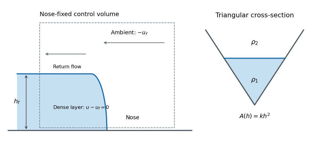
To determine an appropriate coefficient theoretically, take a control volume moving with the nose and bounded by sections far enough ahead and behind for hydrostatic pressure and approximately uniform section velocities to apply. Use the actual triangular wetted areas and integrated pressures. Conservation of fluid volume fixes the ambient return-flow velocities; integrated horizontal momentum balances the incoming and outgoing momentum fluxes against the pressure forces. A Bernoulli relation on an ambient streamline, with an explicit nose-loss assumption if needed, supplies the pressure or energy closure. The density-anomaly pressure contribution of the lower layer contains the integral derived above. Solving those balances gives and hence .
Alternatively, measured front speeds and consistently defined adjacent heights in a geometrically similar experiment can calibrate the closure. A rectangular-channel numerical coefficient must not be transferred to a triangular channel without checking those balances. The height definition and dissipative nose structure also matter; a primary study of gravity-current front conditions explains why different height conventions can lead to different inferred coefficients. No numerical value of is required for the following solution.
Let , as printed in the PDF. The converted TeX misrenders this expression. The undisturbed reservoir has , . The expansion fan moving into it is a simple wave with constant. On the other characteristic family, a self-similar fan satisfiesSolving these two equations givesThe fan begins at , where it matches the initially resting reservoir.
At the front, write . The nose closure is and the invariant gives . ThereforeA uniform region of this state connects the right edge of the fan, , to the advancing front . Its width is . The complete lower-layer solution for isandAhead of the front there is no lower-layer current, so its velocity is not a physical variable there. Both transitions inside the current are continuous; the finite-height nose is closed by the ambient-front condition, not by an unsupported vacuum jump. These formulas give the front-regularized triangular-channel dam break for any specified positive constant .
Initially the same expansion fan and constant-speed front apply. Its left edge reaches the closed rear wall at . After that, the infinite-reservoir solution would give a nonzero velocity at the wall and violates the no-through-flow condition. A reflected disturbance adjusts the interior while the finite initial volume is progressively spread over a longer, shallower current.
The nose does not respond instantaneously when the fan reaches the wall. Its first return signal follows a characteristic from through the undisturbed fan. There , so integrating givesIt reaches the uniform nose-adjacent region at , where . Crossing that region at speed , it catches the front at . Thus the initial nose remains uninformed about the rear wall until this return time. Subsequently its speed must adjust rather than remain constant indefinitely.
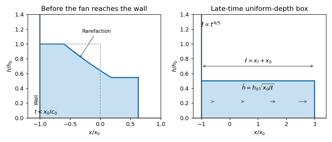


For late times use a prismatic triangular-channel gravity-current box model with uniform representative depth over length . The initial volume is . With no entrainment or loss,Apply the same front closure using that representative depth:Starting from a matching late-time state , integration gives finite-volume inertial spreading in a triangular channel:Hence , and the nose speed decays like . A simple initialized box approximation can instead set and , but it then deliberately replaces the exact early rarefaction rather than reproducing it.
The box's volume equation is compatible with a velocity increasing linearly from zero at the rear wall to the nose speed: . A flat-depth box with this velocity is not an exact solution of the full momentum equation during deceleration. It is an integral approximation that leaves the interior shape and nose dynamics unresolved while predicting late-time bulk scaling.
Write and average the horizontal Navier-Stokes equation, with zero-mean fluctuations and incompressible flow. The mean flow is stationary, has no vertical velocity and has no horizontal pressure gradient. The mean advection of is therefore zero. Incompressibility rewrites the averaged nonlinear fluctuation term as a divergence:These correlations transport mean momentum and produce Reynolds stress. Horizontal statistical homogeneity makes the horizontal derivatives of the averaged correlations vanish. It does not require the instantaneous turbulent derivatives themselves to vanish. Only the vertical divergence remains, givingMultiplying by density and integrating once gives constant-stress Reynolds-averaged wall flow:Here is physical shear stress. Positive mean shear commonly has , representing downward transport of positive horizontal momentum. The Reynolds term then contributes positively to the total stress.
The printed target formula has an extra vertical derivative in the Reynolds contribution. That term has dimensions of stress per length, while has dimensions of stress, so the formula as printed is inconsistent. The derivative belongs in the stress-divergence equation above; the boxed integrated stress is the corrected result. Part b also uses a kinematic rather than physical stress, so the density factor must be tracked explicitly.
Define the friction velocity for positive wall shear. In the near-wall region turbulence is suppressed and molecular viscosity carries the stress. With no slip, . The viscous wall coordinate becomes order one at the characteristic viscous sublayer lengthThe numerical extent of viscosity dominance depends on the crossover convention and wall condition; the scaling is the required viscous length.
An eddy at height cannot extend arbitrarily far through the ground, so its largest local vertical scale is proportional to . Choose and absorb its constant of proportionality into the coefficient. With the prescribed constant turbulent velocity scale, writeThe mixing-length closure is . Thus the full kinematic stress isFor , neglect the molecular term. With no internal momentum source, is constant, soIntegrating between two heights givesEquivalently define an extrapolated roughness length and write . If , the familiar law of the wall is . The logarithmic profile is valid outside the inner viscous region and below scales where the constant-stress or wall-distance assumptions fail. It cannot be continued to to impose the smooth-wall no-slip condition.
The part b notation must therefore mean , a stress divided by density. Using the physical stress from part a on that right-hand side would omit a factor of .
The turbulent Schmidt number compares turbulent momentum and concentration diffusivities:The mean fluid has no vertical velocity. Taking positive upward and , the settling flux is , while the given turbulent particle flux is . Local particle-volume conservation therefore givesConsequently the evolution equation isFor constant settling speed this is . In the logarithmic region, from the preceding part. The sign is consistent with downward settling: without diffusion, a profile evolves as . The dilute suspension approximation neglects feedback on the mean flow and particle interactions; deposition or erosion must be imposed through the bed boundary flux.
Particles settle toward the bed under their submerged weight. A concentration increasing downward gives an upward turbulent diffusive flux, which can oppose that settling. If turbulence cannot sustain the particles, they enter the weakly mixed near-wall region and can deposit. Sediment resuspension requires bed forces strong enough to entrain grains, not merely a specified diffusivity far above the bed.
For noncohesive grains, an appropriate criterion uses the Shields parameterwhere is grain size, its density and the sediment entrainment threshold expressed dimensionlessly. The threshold depends on grain geometry, contacts and viscous effects; cohesion changes the criterion. Sustained suspension additionally requires sufficiently vigorous upward turbulent motions relative to . Bed motion and well-mixed suspension are therefore not identical conditions.
At sedimentation-resuspension equilibrium, the total vertical particle flux is constant. Set with . The stationary equation givesSince and at infinity, necessarily . Settling and upward diffusion then balance pointwise. Taking a reference height in the specified length units gives the equilibrium settling-diffusion profileIt is nonnegative and decays to zero. The profile describes the region ; it does not assert that this power law continues through the viscous layer down to the physical bed. The supplied reference concentration summarizes the bed exchange and near-wall physics that the outer diffusion closure does not resolve.
The Batchelor entrainment hypothesis makes the inward entrainment velocity proportional to the local plume speed:where is the dimensionless entrainment coefficient. For an upward plume , this is . The hypothesis represents turbulent ingestion of ambient fluid; it is a closure rather than a consequence of mass conservation.
Let , suppressing the common factor from cross-sectional integrals. In the Boussinesq approximation, use a constant reference density in the leading-order mass conservation equation. Dividing that equation by gives volume conservation:The factor two is the ratio of the perimeter to the suppressed area factor . Density differences are retained in buoyancy, even though they are neglected in the leading inertial and volume terms.
To derive the density-deficit balance, first leave the small density differences explicit in the supplied mass equation. Because the ambient density is time independent, the product rule givesThus the ambient mass entrained through the perimeter cancels exactly against its contribution to the volume budget, yielding the required buoyancy balance. It is understood to the accuracy of the underlying Boussinesq approximation; the volume equation is not an additional exact constraint on a fully variable-density fluid.
For later use define reduced gravity and the squared buoyancy frequency . With and , the balance isA stably stratified ambient has , so upward motion consumes the plume's positive density deficit; an unstable ambient reverses this sign.
Use the conventional kinematic plume fluxesThen is the volume flux, the dimensional mass flux, the dimensional momentum flux, and the kinematic buoyancy flux. Calling a mass flux uses a density-normalized convention: the reference density has been suppressed. If density-weighted momentum and buoyancy fluxes are desired, multiply and by the same constant throughout. Here the conventional kinematic definitions make the Boussinesq approximation explicit.
For an upward plume with , the inverse relations areThe volume conservation, vertical momentum conservation, and buoyancy balances from part a becomeHere the vertical momentum conservation equation uses in the inertia and retains in the buoyancy force. The ambient has no imposed vertical momentum at entrainment.
To classify the resulting partial differential equations, work in the nonsingular primitive variables with . Subtract times the volume equation from the momentum equation and times the volume equation from the buoyancy equation. This givesThe principal matrix is thereforeAll three characteristic speeds are real and equal to , so the model is a hyperbolic system if that term means only reality of the characteristic roots. However, for , requires , leaving only two independent eigenvectors. HenceThis weak hyperbolicity of the unsteady top-hat plume prevents a complete set of independent characteristic fields. For example, freezing in the homogeneous principal part gives and . A Fourier perturbation of wave number therefore produces a term proportional to in . Real characteristic roots alone do not provide uniform control of high-frequency perturbations. The flux-variable transformation above is invertible in the stated region, so changing to does not remove this degeneracy.
For a steady upward plume with prescribed , the kinematic plume fluxes satisfyThe positive sign in the last equation expresses the gain of buoyancy flux as the plume rises through the prescribed unstable ambient. Seek a positive power law solution , , , with . Matching powers givesThe last relation gives and the first . Substitution into the middle relation yields , henceThe amplitude equations areFrom the first relation , while the last two give . Taking positive amplitudes gives , and consequentlyReconstructing the radius, speed and reduced gravity gives the top-hat plume in constant unstable stratification:As a direct check, and , while .
The corresponding ambient gradient is . Thus ; for a linear ambient this is . The plume is locally lighter than the ambient even though both densities increase upward in this prescribed unstable stratification.
The coordinate can be measured from a virtual origin. This exact power law branch has fluxes tending to zero there and describes buoyancy generated by the maintained unstable ambient; it does not impose arbitrary nonzero source fluxes at that origin. The given idealization holds the ambient quiescent despite its static instability. Finally, the Boussinesq approximation limits the modeled height range to small relative density changes, here . Within these assumptions, the displayed positive branch proves the requested existence.
Articles by others on the same topic
There are currently no matching articles.