A phase diagram locates stable pure thermodynamic phases and their phase coexistence boundaries in a space of control parameters. For a concrete three-dimensional example, take the temperature, crystal-field parameter, and magnetic field of the Blume–Capel model. Its spins take values ; changing the cost of the zero-spin state can turn a continuous ordering transition into a discontinuous one. A local scalar description near the resulting tricritical point is the Landau-Ginzburg theoryThe three local control coordinates are , with varying linearly with the thermal scaling field. For , , the transition at is continuous. For , zero-field coexistence is at , and the magnetization jumps between zero and . The two loci meet at , the tricritical point.
The full three-dimensional phase diagram has an ordered coexistence sheet at , where the two opposite magnetizations exchange stability when changes sign. On its three-phase line it meets two nonzero-field tricritical wings. These wings are first-order phase transition surfaces between minima of the same sign but different magnitude, terminating at ordinary thermodynamic critical points. Their tricritical wing critical edges are found by :Indeed fixes , and substituting into and gives ; ensures a stable critical quartic minimum. The two signs give the two wings. All transition surfaces and critical edges end together at the tricritical point. The following plot uses ; its wing surfaces come from the exact tricritical wing coexistence factorization, rather than schematic unconstrained surfaces.
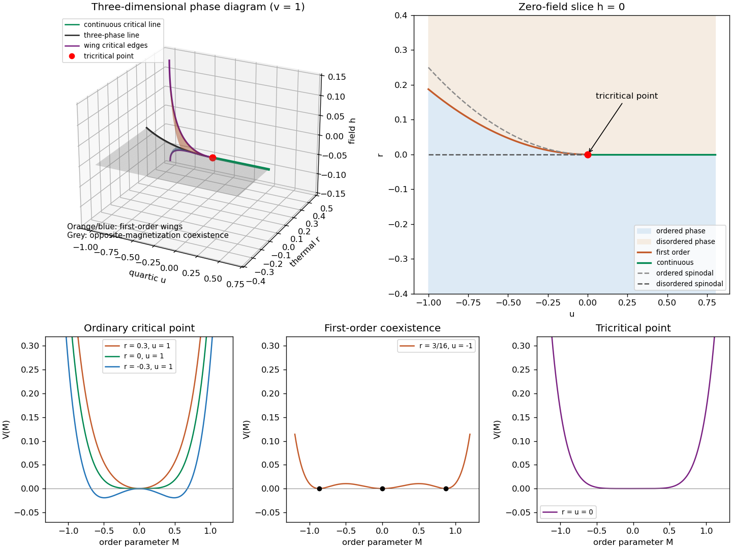
Tricritical coexistence surfaces, the zero-field phase diagram, and ordinary, first-order and tricritical Landau potentials
. Details. 
The unheaded requests for critical exponents follow from the uniform equation of stateFor an ordinary thermodynamic critical point, is fixed and , . At , , the small ordered minimum obeys , so the order-parameter critical exponent is . Above the transition , giving the magnetic-susceptibility critical exponent . At , , so the critical-isotherm exponent is . At the tuned tricritical point, , instead below the transition and on its critical isotherm, while the disordered susceptibility remains . ThereforeBelow the transition the inverse susceptibility is , giving in the ordinary limit and in the tricritical limit. Thus both sides give the same susceptibility power, with different amplitudes.
To derive the general Ginzburg criterion, tune away all lower even nonlinearities and let the leading stabilizer be , . The equation of state gives , and its curvature at the ordered saddle is , so . The fluctuations of the order parameter averaged over a correlation volume are estimated by its long-wavelength quadratic covariance:The integral has a fixed dimensionless upper limit after ; this is a coarse-volume fluctuation estimate, not the ultraviolet-dominated point variance. Consequently the multicritical Ginzburg ratio isThe Landau approximation is asymptotically controlled by this test only when the ratio tends to zero. This gives the upper critical dimensionThe same threshold follows by giving its Gaussian engineering dimension : the coupling to has scaling exponent , which becomes relevant below .
For , the fluctuation ratio diverges and the saddle calculation cannot predict the generic interacting critical exponents. At the test is marginal, not a proof of changed power exponents: the ratio has zero thermal power and marginal interactions can produce logarithmic corrections. Thus the PDF's inclusion of equality in a blanket claim about wrong power exponents needs this qualification. The Landau-Ginzburg theory as a fluctuating field theory remains useful; what loses validity is its fluctuation-free Landau approximation.
An order parameter distinguishes phases by an equilibrium expectation value. For an Ising model, the local field is the coarse-grained magnetization, and the uniform value is . The spin inversion symmetry maps to , so at zero field the Landau free energy contains even powers. Its disordered minimum is ; ordered pure thermodynamic phases have . Their sign is selected by taking the thermodynamic limit before sending to zero. A symmetric mixture can have zero average without being a single disordered phase. The term identifies as the field conjugate to an order parameter.
Use the connected correlation function in a selected pure thermodynamic phase. The exponential correlation length is defined by , when this limit exists in the chosen direction. Linearizing the Landau-Ginzburg theory around a stable uniform minimum givesHence the Landau scalar correlation length is . Away from criticality the massive Gaussian field correlation tail behaves as , up to its amplitude. At a continuous transition tends to zero, so diverges and fields vary on scales much longer than the lattice spacing. This motivates a gradient expansion, but the simultaneous growth of correlated fluctuations is precisely why the Ginzburg criterion must be checked.
A first-order phase transition exchanges distinct global minima of the Landau free energy; the order parameter jumps and a thermal crossing generically has latent heat. A continuous phase transition has minima merging continuously and a diverging correlation length. A local loss of stability at a spinodal point is not the equilibrium coexistence condition.
For the sextic even Landau potential, write . At a nonzero zero-field stationary point, . To coexist with , also require . Eliminate to obtain and , which requires . On this locusproving that all three equal minima are globally stable. Their curvatures are at zero and at the nonzero minima, so the correlation length is finite when is fixed. For , by contrast, the nonzero minimum approaches zero as , giving the ordinary continuous transition. At fixed and , crossing exchanges the two ordered minima discontinuously even though the zero-field thermal transition at is continuous.
Universality classes identify systems with the same long-distance renormalization-group fixed point. Spatial dimension, order parameter symmetry and number of components, and the range of interactions help determine the equilibrium class. Microscopic lattice details and many local interactions become irrelevant operators under coarse-graining. Universal quantities include critical exponents, scaling functions after fixing metric normalizations, and suitable amplitude ratios. The critical temperature, bare couplings, absolute correlation-length and susceptibility amplitudes, analytic free-energy density backgrounds, and microscopic length scales are generally not universal. Dynamic universality can additionally depend on conservation laws, so it should not be inferred solely from a static scalar potential.
A critical exponent describes the leading singular power of an observable in a specified scaling limit. The order-parameter critical exponent describes the zero-field ordered branch; the magnetic-susceptibility critical exponent describes response to its conjugate field; and the critical-isotherm exponent describes response at the critical temperature. They are found in the Landau approximation by minimizing the potential and differentiating the resulting equation of state, as calculated in the question's root solution. For a leading stabilizer the same calculation gives , and . Thus , and . Beyond the Landau approximation, the renormalization-group relevance exponents and anomalous dimension determine the singular powers; Question 2 derives their relations. The critical exponents refer to specified paths, and tuning to a higher multicritical point requires eliminating its lower relevant perturbations.
At a tricritical point, both and vanish, while stabilizes the Landau free energy. It separates ordinary continuous transitions for from first-order coexistence for . The zero-field order-parameter jump shrinks to zero as , and the tricritical wings terminate there in the full diagram. For , , minimizing gives andTwo thermal derivatives give the heat-capacity critical exponent , compared with the finite mean-field heat-capacity jump, , at an ordinary quartic transition. The remaining tricritical mean-field critical exponents are , and the mean-field correlation-length critical exponent is . To observe tricritical scaling one must tune the quartic scaling field as well as the thermal field: a generic path with fixed instead has ordinary critical behavior. Its upper critical dimension is three, as the multicritical Ginzburg ratio shows.
Use for inverse temperature, to distinguish it from the order-parameter exponent. In a translation-invariant pure thermodynamic phase, the connected correlation function isThe subtraction is essential below the transition. Its exponential correlation length is defined by , with direction specified if the lattice is anisotropic. Away from criticality, has a tail proportional to times an algebraic prefactor. In the massive continuum scalar approximation that prefactor is ; at criticality the exponential cutoff disappears and instead. The large-distance limit here is , as the PDF shows.
Let . With the energy convention , the magnetization per site and magnetic susceptibility areWriting , direct differentiation of the partition function gives . Thus the correlation-function susceptibility sum rule isIn physical continuum coordinates the lattice sum becomes , so omitting the site-density factor would change the normalization. A derivative with respect to the dimensionless source instead absorbs the explicit inverse-temperature factor.
An exact renormalization-group transformation with length factor can be defined by a nonnegative normalized blocking kernel satisfying . A deterministic majority rule is one example; randomized tie-breaking preserves its normalization. Define the blocked energy, including its constant, bySumming over proves . All generated operators must be retained for this identity to remain exact; a finite-coupling truncation is an approximation. After iterations, and the spacing is . Long-distance physics is preserved because this is a marginalization of microscopic probabilities, with observables and sources transformed along with the energy. It integrates short-distance variables rather than changing their effects on retained observables. Physical lengths remain fixed even though the correlation length in units of the new spacing is reduced by .
For clarity, now use dimensionless free energy per site . Exact equality of the partition functions givesA constant microscopic energy shifts every blocked weight by the same factor, so . Substitution at one step yields the additive free-energy recursion under blockingInduction now gives the requested relationThe function is the identity-operator contribution to renormalization-group free energy: it records eliminated-mode entropy, integration constants and normalization factors. A free-energy function satisfying this inhomogeneous equation need not be purely singular until its analytic background has been subtracted.
At a renormalization-group fixed point, . Linearize in scaling coordinates so . Here is a scaling exponent, not the discrete multiplier itself. A positive gives a relevant operator, a negative one an irrelevant operator, and zero a marginal operator. The critical surface is the stable manifold: tune every relevant scaling field to zero and the irrelevant coordinates flow toward . A repulsive renormalization-group trajectory leaves along a relevant direction; it can still have irrelevant coordinates contracting toward that manifold. The plot shows the section when temperature and field are relevant: is the critical line in this section, while an independent nonzero field is another direction away from criticality.
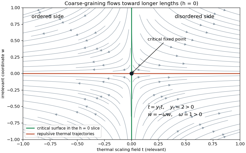
Renormalization-group trajectories near a critical fixed point, showing thermal repulsion and irrelevant contraction in the zero-field section
. Details. 
The inhomogeneous term cannot simply be discarded from the full free energy. If an analytic background solves , its subtraction leaves obeying homogeneous scaling. For example, in linear thermal and field coordinates, a source monomial is removed byWhen the denominator vanishes, the source is resonant and can instead produce a logarithm. Thus the homogeneous singular equation is justified after analytic subtraction when there is no relevant resonance affecting the leading singularity, no marginal logarithm that has been omitted, and no singular dependence on a dangerously irrelevant coupling. Merely saying that is regular is insufficient to discard the whole weighted sum without this analysis.
Under these assumptions, with two relevant scaling fields , choose so that is of order one. The scaling hypothesis for critical phenomena then givesWriting recovers the PDF's notation:The sign labels the two matching branches and , which enter different phases when the flow leaves the critical neighborhood. The constants retain a branch-dependent identity contribution or a chosen split of the scaling function. They are determined by the same matching problem, not independently adjustable nonuniversal free-energy offsets. An arbitrary analytic offset from belongs to the subtracted background. The formula describes the singular part; adding that background recovers the full physical free energy.
At , restore the common metric factors as . Their ratio at equal is , proving the expected universal singular free-energy amplitude ratio because and cancel. The ratio of full free energies including an arbitrary regular is not universal; zero amplitudes and logarithmic resonances also require separate treatment.
The critical exponents are obtained by rescaling and differentiating, not by identifying them with the discrete multipliers. The correlation length obeys , hence . Two temperature derivatives of give , while one and two field derivatives give the ordered magnetization and susceptibility powers. ThusFor , instead set and choose the blocking scale by , obtaining and then differentiate. A nonzero spontaneous ordered-branch derivative is assumed in the formula for . In particular the hyperscaling relation is . Its physical assumption is an order-one singular free energy per correlation volume, with a single diverging length and no dangerous variable changing its volume scaling. Above the upper critical dimension, a stabilizing quartic coupling can invalidate that assumption even though the correlation length still scales.
For the last model, take the quadratic Hamiltonian exactly as visually printed: its source term is , outside the half multiplying the gradient and mass terms. With and , its connected quadratic covariance is proportional toThe pole scale, or the massive Gaussian field correlation tail obtained by its Fourier transform, givesThe uniform source shifts the mean to and does not change the connected covariance. Replacing by matches the earlier magnetic source convention without changing any scaling index.
Define a Gaussian thinning transformation by retaining momenta , integrating the Gaussian shell, and rescalingThe gradient coefficient is unchanged. Counting volume and field powers in the remaining action givesShell integration contributes only the additive determinant term. Thus when the thermal variable is proportional to , and . Inserting these into the homogeneous index formulas gives the requested Gaussian critical exponentsThe specific-heat power can also be verified without hyperscaling: two mass-squared derivatives of produce an integral proportional to . For , rescaling gives ; at the divergence is logarithmic, with power index zero. At the determinant itself has an additive resonance, although its heat-capacity power remains one.
There is a genuine limitation to the last printed request. The Gaussian order-parameter scaling index is formal: a pure quadratic theory has at , and at the uniform energy is unbounded below, so its partition function diverges. It therefore has no stable ordered branch from which a spontaneous-magnetization exponent can be measured. The thinning derivation establishes the index requested by the PDF, but not a nonexistent ordered phase. A stabilizing quartic interaction is relevant for and generally changes these Gaussian indices to the interacting critical ones.
Replace each XY model bond weight by its periodic Gaussian approximation. With angles integrated using , the Villain model iswhere is the number of bonds. Changing the angle-measure normalization multiplies by an explicit constant only. The Poisson summation formula applied to one bond gives the equivalent winding representationThus the same Villain model can be written . The coefficient is the PDF's value; the converted TeX incorrectly places outside the square root. The cosine-to-Gaussian replacement is a large- approximation, but the rest of the calculation treats as the exact model for every positive .
Angle integration gives a dual representation in any lattice dimension. Discrete summation by parts rewrites the phase asEach normalized angle integral is a Kronecker delta. This proves the integer-current representation of the Villain modelThe PDF does not specify dimension or boundaries. The point-vortex vortex Coulomb gas interpretation below is two-dimensional. In three dimensions the defects are vortex lines, and the dual constrained-current representation still holds but is not a gas of point charges with logarithmic interactions.
First take a connected simply connected planar lattice, with free outer angles, so no torus winding sectors are silently discarded. Assign an integer height to each dual face, fixing the exterior face height to zero. A divergence-free integer current is exactly the oriented height difference on the two faces adjoining its bond. To see existence, integrate the rotated current along a dual path: the change around a closed dual path is the total divergence inside, hence zero. Integer currents give integer heights, and fixing the exterior removes their constant-shift ambiguity. Thereforewhere is the positive dual graph Laplacian with the exterior height fixed. This gives the dual integer-height representation of the planar Villain model.
Apply the supplied Poisson summation formula separately to every interior height. For interior faces,Complete the Gaussian square, or use its characteristic function, to evaluate the integral asThus the smooth fluctuations and integer defects separate:The Gaussian factor is . It really is the spin wave factor of the original lattice: the planar Euler identity gives , and the matrix-tree theorem identifies with the spanning-tree count of the original graph. Its reduced primal Laplacian has the same determinant, so the noncompact Gaussian angle integral with one angle fixed has exactly this prefactor. The compact common-angle mode has been normalized to one. The remaining variables are integer vortex windings on the faces, giving the vortex Coulomb gas.
For periodic boundaries, has a zero mode, and there are also two noncontractible current sectors. Neutral charges use the inverse on the mean-zero subspace. An integer dual height may have twists across periods . Subtracting makes the remaining height periodic; the gradient energy gains . Its height Poisson summation supplies the phase , where and . A second Poisson summation in yields the positive harmonic-sector factor in periodic Villain dualityUp to charge-independent normalization, the exact periodic result is . Smooth spin waves still factor out, but the finite-volume global winding sectors couple to vortex dipole moments. The familiar neutral bulk formula suppresses this boundary information; it must not be asserted as an exact finite-torus formula without specifying those sectors.
At long distances in two dimensions the lattice Green function solves and has . Indeed the flux of through a circle is one, fixing that coefficient. For well-separated vortices at with integer charges , the vortex Coulomb gas action becomeswith the self-energy convention, boundary terms and any global sectors retained separately. The factor two in the pair sum comes from the two ordered terms in . Opposite charges have pair action , so separating them costs energy and they attract. Like charges have a negative logarithmic pair coefficient and repel. The ultraviolet lattice regularizes the core, while multiply charged defects have a quadratic self-energy cost. A separated unit vortex-antivortex pair costs , the energetic basis for vortex-antivortex binding at low temperature. In three dimensions one instead has interacting closed vortex lines with a three-dimensional Green kernel; the logarithmic point-pair formula is specifically two-dimensional.
For a periodic two-dimensional lattice the vortex charge neutrality constraint is . In the winding form of the Villain model, is the oriented plaquette curl of the integer bond variable , up to an orientation sign. Summing all plaquette curls cancels each bond against its neighboring plaquette. This proves neutrality directly. Equivalently, restoring the common dual-height mode modulo its integer shift gives , which vanishes unless the total charge is zero; only then is the inverse lattice Laplacian well-defined on the charge source.
On an infinite plane, the same condition is required for a localized finite-energy configuration with constant phase at infinity. Net charge produces far away, so its exterior action iswhich diverges unless . With an open boundary the total charge instead equals the boundary winding, and the finite planar duality in part (b) can sum nonneutral configurations. Thus neutrality follows from periodicity or the stated finite-energy boundary condition, not from arbitrary boundaries. In three dimensions the analogous local constraint is that vortex lines cannot end in the bulk.
Write for the PDF's signed mass coordinate , and . The superscript on is notation here, not a restriction to positive mass. In a momentum-shell renormalization group step, remove momenta and set , the PDF's . Split the scalar field into a slow field and a fast field , whose Gaussian shell covariance is . The shell must have a positive quadratic kernel; near the fixed point meets this requirement.
Expand the coarse action by the cumulant expansion of a coarse-grained free energy. In the first cumulant of , the term with two fast fields is . Thus the one-loop shell mass renormalization in scalar quartic theory isFor the quartic correction, the two-fast-field vertex is . Its connected second cumulant has a minus sign and uses . It givesTaking the local zero-external-momentum quartic part produces , where . This derives the combinatorial factors in the one-loop shell quartic renormalization. The mass tadpole is independent of external momentum; kinetic normalization changes only at higher order for the leading epsilon calculation.
For an infinitesimal spherical shell, radial integration givesLowering the cutoff adds the engineering terms and to the running dimensionless couplings. Since and , the remaining cutoff powers cancel exactly. ThereforeThese are the requested flows, to the stated one-loop order. They implement cutoff independence of long-wavelength observables after changing the couplings and retaining the generated constant and other effective operators to the relevant approximation order. They are not an exact closure of the complete effective action.
Besides the Gaussian fixed point, solve the nonzero-coupling fixed-point equations. The quartic equation gives . Substitute into the mass equation to get , hence within the displayed one-loop truncation. Since ,These are the Wilson-Fisher fixed point coordinates in this cutoff scheme. The higher terms obtained by solving the truncated equations exactly should not be regarded as a full higher-order epsilon calculation.
The attraction claim in the PDF needs a thermal qualification. The stability matrix of a renormalization-group fixed point at this solution has entriesThe lower-left entry is , so its eigenvalues areIncreasing means approaching the infrared. The quartic scaling direction is attractive, but a perturbation in the thermal scaling direction grows as . Therefore the Wilson-Fisher fixed point is an infrared attractor on its tuned critical surface, not an attractive fixed point of the entire two-dimensional coupling plane. In the plane it is a saddle; an arbitrary small thermal perturbation is a concrete counterexample to unconditional attraction. This is the thermal relevant direction at the Wilson-Fisher fixed point.
For , the quartic interaction has a nonzero limiting value instead of disappearing under coarse-graining. Long-wavelength thermal fluctuations are therefore interacting, so the fluctuation-free Landau approximation cannot give the generic critical powers. For example, its ordinary correlation-length critical exponent is , whereas the relevant thermal eigenvalue just derived givesThe tadpole is momentum independent, so the anomalous dimension begins at . Combining this with the scaling relations yields , , and , exhibiting the deviation from ordinary mean-field indices. These are controlled statements for small positive , not exact numerical exponents at arbitrary dimension. The Landau-Ginzburg theory itself is not invalid: integrating its fluctuations is precisely how the Wilson-Fisher fixed point was obtained. The invalid step is replacing that interacting long-distance theory by a uniform saddle and ignoring its fluctuation corrections.
Articles by others on the same topic
There are currently no matching articles.