The characteristic polynomial factors as , so the complementary solution is . Each exponential forcing resonates with a homogeneous mode; the method of undetermined coefficients therefore uses and . Substitution gives the particular solution . ThusThe initial conditions give and . HenceThe factors of in the particular solution are essential: an unmodified exponential trial lies in the kernel of the differential operator.
Set . The chain rule gives , so the transformed equation is the forced harmonic oscillator , with and . ThereforeThis real solution is defined only where its logarithm has positive argument. Put and . Then , and the connected interval containing zero is .
Since , a stationary point requires . The positive branch cannot contain the oscillator minimum . It contains the maximum , attained first at . HenceAt the endpoints where , tends to minus infinity; the oscillator solution cannot be continued through those zeros as a finite real .
Expand around the expectation :Thus variance as the minimum mean squared error of a constant givesThe finite second moment also guarantees the finite first absolute moment needed below.
For a probability density function , splitting at givesLet be the cumulative distribution function. Since a density gives no mass at a singleton, differentiating under this integral yields . This derivative is nondecreasing, so is convex andThis is the median minimizes expected absolute loss property. The minimizer need not be unique: a gap in the density can give an interval of medians, all with the same loss.
For , monotonicity gives . Apply Markov inequality to the nonnegative variable :If the expectation is infinite, the bound remains true but uninformative. At the right side is one, so that endpoint follows directly. Minimizing over gives the Chernoff bound.
The Poisson distribution with unit parameter has mass . Its moment-generating function isFor an integer , multiply the exponential probability bound by to obtain . The exponent is minimized at , hence , including when . Consequently
For the normalized second-order equation, an ordinary point is one where both coefficient functions are analytic. A singular point of a second-order linear ODE is a point that is not ordinary. It is a regular singular point if and extend analytically to ; a singular point failing that condition is irregular.
Here , . Thus zero is singular but regular, because and are analytic. Write the analytic solution as . Its constant equation gives , and for ,Using givesThe factorial denominators show convergence for every finite .
For the other branch, integrating the first correction equation twice and imposing its two conditions gives andThen , so andEach correction tends to zero at the origin and its derivative vanishes at one. Although the second solution has a finite limiting value one, it has a logarithmically divergent endpoint derivative. Indeed the differential equation gives , and integration givesA finite initial derivative cannot be prescribed for this second branch. The logarithm is consistent with the integer separation of the two exponents in the Frobenius method; this is not the repeated-exponent case.
Expand the function into separated terms: , where and . ThenPut and . The nine critical points are all pairs from and . The diagonal Hessian matrix has entries and .
At both entries are positive, giving strict local minima of value . At they have opposite signs, giving four saddle points of value zero. At the three points on the Hessian is degenerate, so its sign alone does not classify them. Use the higher-order test for separated extrema: is negative for small nonzero . At the positive term and negative term give a saddle. At , , so every sufficiently small nonzero displacement decreases and these are strict local maxima.
For the level curves, the exact zero set consists of the two parabolas and the oval . They cross at the four nondegenerate saddle points. Small positive levels enclose each maximum; small negative levels enclose each minimum. The degenerate central saddle has quartic narrowing, locally . Far along the axis the function is negative, while far along the axis it is positive. These signs and zero curves determine the connectivity shown in the sketch.
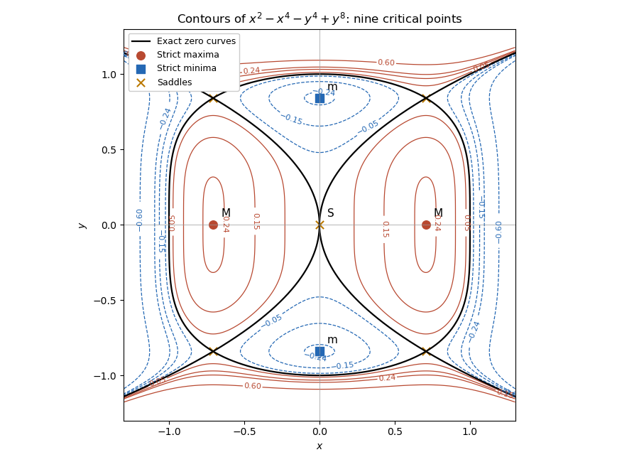
Level curves, exact zero set and all nine classified critical points of the separated quartic-octic function
. Retain the derivative marks and coefficients from the printed system. In matrix form it is , withSince , multiplication by its inverse givesThe linear transformation , diagonalizes this system:Both start at zero. An integrating factor gives , soDirect substitution into the two original equations confirms the different forcing coefficients; the exact cancellation in depends on those coefficients.
Let , with . Newton law of cooling gives the warming and cooling profilesIn the stipulated linear model, . The bacterial count obeys , so its logarithmic reduction is the cumulative thermal destruction under exponential warming and cooling:Writing , the warming integral divided by is and the cooling contribution is . Hence the required implicit equation isThe bracket is zero at zero and has derivative for , tending to infinity with . There is therefore one positive solution.
For the hardier species, is unchanged in this model if and the achieved remain the same. Raising the oven temperature changes , but its factor cancels against the changed slope of the linear destruction law. The entire normalized temperature history and hence the destruction integral remain the same; the comparison uses both the warming and equal-duration cooling stages.
The exponential distribution has survival probability for . Conditional probability therefore giveswhich proves the memoryless property. Let and . With ,The geometric distribution here starts at zero. Summing its first moment givesFor , sum the density over all integer translates:with zero density outside that interval. The integer and fractional parts of an exponential variable are independent, because for every integer and measurable ,This factorization proves independence of the discrete and continuous components, beyond just checking their separate marginals.
For the probability generating function , differentiation givesThe second derivative is a factorial moment, not the raw second moment.
In the Galton-Watson process, condition on . The next generation is a sum of independent offspring counts, and so its conditional generating function is . Averaging over givesThe conditional mean is and the conditional variance is . Thus iterated expectation gives from one ancestor, and the law of total variance gives , . Iterating yields the branching-process generation momentsFor the critical case , the correct limiting value is . If , nonnegative offspring are zero almost surely, so every later generation has zero mean and variance; handle this directly rather than use an ambiguous zero power. At generation zero the mean is one and variance zero.
The branching-process extinction criterion states that extinction probability is the smallest fixed point of in : probabilities of extinction by successive generations are the iterates of from zero, increasing to that fixed point. Here the equation is , factoring as . The two admissible roots are and one, so
Use the positive-support geometric distribution, for , . Differentiating the geometric series suppliesFor the jar, let be the waiting time to remove one red ball when exactly red balls remain. Every draw has success probability , so is geometric with that parameter. The are independent: after each success, fresh independent draws begin a new stage, and its conditional waiting distribution depends only on the deterministic count , not on earlier waiting times. Replacing a green ball leaves that stage's count unchanged.
Thus the coupon collector problem decomposition is , andThis is the coupon collector waiting-time variance. For , the formula correctly gives zero variance and a deterministic one-minute completion.
By the partition and the law of total probability, . Also . Combining these identities proves Bayes theorem:The assumed positive probabilities make the conditional expressions well defined.
Let mean that the selected coin is biased and that it is fair. Both have prior probability . Conditional on either coin, tosses are independent. For the observed head count, the two binomial distribution likelihoods are and . Bayes theorem cancels the common coefficient and equal prior weights, givingThis applies for , including endpoint coin biases with zero-power factors interpreted by the corresponding likelihood. The fair-coin likelihood is positive, so the denominator cannot vanish.
For a finite stopping time with target , necessarily . The last toss must be a head and the preceding tosses must contain heads. The negative binomial stopping argument therefore gives likelihood for the biased coin, and for the fair coin. Applying Bayes theorem again yieldsThe two experiments have different combinatorial coefficients, but each coefficient is independent of the coin parameter. Thus posterior equality for proportional likelihoods explains their identical posterior formula. If , a finite positive-head stopping observation has zero likelihood under the biased coin, consistently giving posterior zero. If the target is , the experiment stops at without a toss and the posterior remains ; a positive stopping time would then be impossible.
Articles by others on the same topic
There are currently no matching articles.