De Moivre's theorem states that for integer . For , write its polar form as , where . If and , equality of moduli gives and equality of arguments gives . Thus the distinct roots of a complex number areChanging the chosen argument of only permutes these roots. For the only root is zero. Taking and gives the cube rootsCubing any of them returns ; geometrically they are equally spaced on the circle of radius two.
Put . Squaring the two nonnegative moduli and expanding gives . Completing the square yieldsThus the locus is an Apollonius circle with center and radius . No extraneous points were introduced by squaring, because both original sides are nonnegative. Its intersections with the imaginary axis are and , useful landmarks for the sketch. It surrounds zero but does not pass through zero:
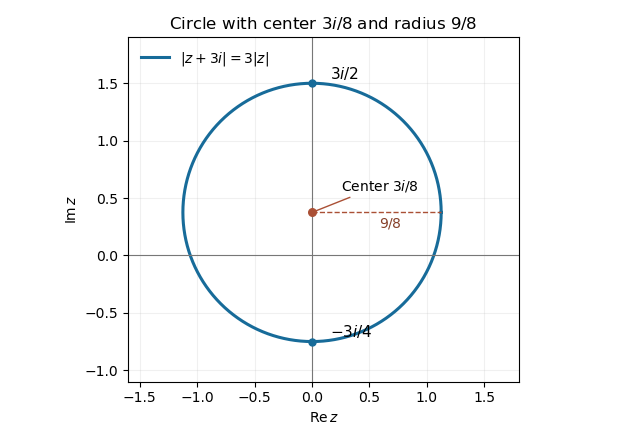
Apollonius circle centered at three eighths i with radius nine eighths and imaginary-axis intercepts minus three quarters i and three halves i
. Left multiplication by the given Givens rotation mixes rows two and three, so . If , chooseEquivalently modulo . Substitution gives and . If , take ; the desired zero is already present. This also covers singular matrices without division by zero.
The second Givens rotation leaves row three unchanged, so . Its other relevant entry is . For , takeThen and . If both entries vanish, choose . The first column now has zeros below its diagonal.
Rows two and three of both have zero in column one. Any rotation of these rows therefore preserves those zeros, so . In column two, . For , chooseThis gives . Again choose if both relevant entries are zero. Thus the successive Givens rotations have eliminated all entries below the diagonal without recreating earlier ones.
Each plane rotation satisfies . Hence is an orthogonal matrix and is an upper triangular matrix. Multiplication by gives the QR decompositionThe zero-pair cases already handled make this construction valid for every real matrix, including rank-deficient matrices. Orthogonality follows from the product identity, not from any invertibility assumption on .
Write and . Expanding the product produces and additional nonnegative terms, giving . Applying the exponential inequality to every factor givesBoth sequences are increasing, since the terms are positive. If converges to a finite value , then , so the convergence theorem for monotone bounded sequences makes converge. Conversely, if has a finite limit, then is bounded and increasing, hence converges by the same theorem. Thus the positive series and the product both converge to finite limits, or both diverge to . This proves the positive sum-product convergence criterion. The word limit here means a finite real limit; allowing extended infinite limits would make the conclusion vacuous for these monotone sequences.
Let . Pairing consecutive terms shows andThe even partial sums increase and the odd partial sums decrease. They satisfy , whileBoth are monotone bounded sequences and hence have limits, and the displayed difference makes their limits equal. Every partial sum belongs to one subsequence, so the alternating series converges. This is a proof of the alternating series test; the monotonicity and zero-limit hypotheses play separate roles.
The summand is positive, so it suffices to show that its partial sums are unbounded. On the block , for ,There are terms in that block, so its sum is at least . Adding blocks gives a constant multiple of the divergent harmonic series. HenceEquivalently the integral test for convergence gives . The block proof supplies the divergence without assuming the integral test.
Two nonzero vectors are linearly independent when forces . Their linear span then has dimension two. If they are linearly dependent, one is a nonzero scalar multiple of the other, and their span has dimension one. Thus the two requested dimensions are .
The Euclidean scalar product and its norm are and . To prove the Cauchy-Schwarz inequality, first handle trivially. Otherwise the squared normgivesEquality holds exactly when the residual vector is zero, meaning the vectors are linearly dependent; this includes the zero-vector cases. Expanding and applying Cauchy-Schwarz then givesTaking nonnegative square roots proves the triangle inequality.
For the unit-vector optimization, let . Independence ensures . The variable part of is , which Cauchy-Schwarz bounds below by . Equality occurs only for the antiparallel unit vector. ThusThis is minimizing a linear functional on a sphere. The two consequences follow below.
The triangle inequality gives . Taking its negative reciprocal givesIn fact independence excludes the equality case , so the inequality is strict under the stated independence hypothesis. The weaker requested bound holds for every permitted pair.
When , the squared norm of their sum is . ThereforeThe minimizing vector is indeed a unit vector. All three pairwise scalar products then equal , so these three unit vectors lie in a plane, separated by degrees.
For a linear map , its kernel and image of a linear map areThe kernel is a subspace of the domain and the image a subspace of the codomain. Given the stated bases, define the matrix of a linear map byIts th column is the coordinate vector of ; if , the output coordinates are .
For the change of basis, write and . The matrices are invertible. Input coordinates change by and output coordinates by , soThe domain and codomain basis changes need not be the same matrix.
For , the two input vectors form a basis of , so its image is the span of and . The vector is orthogonal to both, since . Every possible output therefore satisfies , whereas the target itself is and . Hence there is no with the required output. This uses an image obstruction by an annihilating functional, rather than an inconsistent guessed input.
For , use the input basis , , . Its determinant is , so it is genuinely a basis. Write . ThenSubstitution back into physical coordinates givesFor a direct check, its standard matrix is , which annihilates exactly that line.
We prove independence of eigenvectors for distinct eigenvalues by induction on the number of vectors. A single eigenvector is nonzero and hence independent. Suppose the first are independent, and let . Applying givesBy the induction hypothesis every coefficient in this shorter relation vanishes. The eigenvalues are distinct, so for . The original relation becomes , and gives . Thus the entire family of eigenvectors is linearly independent. The argument works over either the real or complex field.
Represent the quadratic form by the symmetric matrixThe block has characteristic polynomial . Corresponding orthonormal eigenvectors, together with the direction, areThe eigenvalues are . To eliminate the linear term, solve , obtainingIndeed the first equation gives , and the second then gives . Define the new coordinates by . The original polynomial takes the value at the center, so its translated and orthogonally diagonalized form isThusThe surface is an elliptic one-sheet hyperboloid, centered at , with axis parallel to . Its waist at is an ellipse with semiaxes and . Every constant- section is a nonempty ellipse, so the two signs of belong to the same connected sheet. This is an application of principal-axis reduction of a quadric.
Construct the matrix of a linear map by expressing the images of the basis vectors in that same basis:Thus the th column is . For , linearity givesThe column is a coordinate vector; reconstructing the actual vector requires . This distinguishes the linear map from its basis-dependent matrix.
By the given matrix similarity, for an invertible . HenceThe characteristic polynomials are identical. Therefore the characteristic equations and eigenvalues, including algebraic multiplicities, agree. The conclusion is independent of the choice between and conventions.
Rescaling the first basis vector gives the change-of-basis matrix , invertible because . Direct multiplication givesThus the matrices are related by matrix similarity. In terms of basis images, the coefficient along the rescaled first basis vector is divided by , while the second component of its image is multiplied by .
Let the repeated eigenvalue be , and choose an eigenvector . Complete it to a basis of . In this basis the matrix is an upper triangular matrix, with first column , say . Its characteristic polynomial is . By part (a)(ii), this must equal , so .
If , the matrix is already . If , rescale the first basis vector by and apply part (a)(iii); the upper-right entry becomes one. ThusThe second possibility is a size-two Jordan block. It has only one independent eigenvector, whereas has a two-dimensional eigenspace, so the two types cannot be related by matrix similarity. This repeated-eigenvalue classification in dimension two proves the required result without assuming the general Jordan normal form theorem.
Use the orthonormal right-handed basisDirect multiplication gives , and . Thus the matrix in this basis isThe last two columns are orthogonal and both have squared norm . Therefore is an orthogonal matrix precisely when , giving the unique positive valueIts determinant is , so it is a proper rotation matrix, not a reflection. The transverse block has cosine and sine both . ConsequentlyWith the oriented axis , the angle is positive by the right-hand rule, since . The axis also follows from the unit-eigenvalue eigenspace. As a check, .
For a nonzero , the absolute successive-term ratio in the exponential series is , so the first series converges for every . For the factorial series the ratio is , so its terms fail to tend to zero for every .
The third series is sparse: its exponent is , as in the PDF. If , thenFor , the terms grow without bound; at their moduli are , so they again fail the term test. Equivalently, the Cauchy-Hadamard theorem for the sparse coefficients uses , not . Thus the three radii of convergence areZeros at non-square coefficient indices do not change the relevant limsup in the last root test. This illustrates the radius of convergence of a sparse power series.
The Taylor theorem with Lagrange remainder says that, if has continuous derivatives on the interval joining and , then for some strictly between them,More generally the expansion is about any base point, replacing by its displacement. The displayed regularity is a sufficient hypothesis for the theorem.
For and , repeated differentiation givesTherefore the requested coefficients are . For a fixed , the remainder hasNow and for , so . Hence . Passing to the limit proves, rather than merely formally suggests, the binomial seriesThe restriction makes the remainder bound especially direct, since .
Suppose continuity at failed. The negation of the relative-domain epsilon-delta definition gives an such that for every there is an with but . Choosing produces a sequence whose image does not converge to , contradicting the hypothesis. Thus is continuous at .
This proves the sequential characterization of continuity in metric spaces. At or , the same argument uses points only in , giving the appropriate one-sided continuity automatically.
The intermediate value theorem states that a real-valued continuous function on a closed interval takes every value between its endpoint values. Explicitly, if lies between and , there exists with . No monotonicity is assumed.
If is a strictly increasing function and , one of or holds. The corresponding strict inequality of function values shows that is injective. Conversely, if , then is impossible and would imply . ThusTogether with strict increase, this says that such a function preserves and reflects the ordering of points.
Fix . Injectivity excludes or . If , the intermediate value theorem on gives a point other than with value , contradicting injective function. If , the same theorem on gives a point other than with value . ThereforeTo prove strict increase, take . If , the displayed endpoint ordering already gives . Otherwise , and the same interior-point argument on the subinterval yields . Hence is a strictly increasing function. This is the interval order theorem for continuous injections; the assumed endpoint order rules out strict decrease.
First prove continuity at . Given , choose with . Surjectivity gives with . Strict increase implies . For ,Thus proves left continuity at . At , choose and use its preimage to prove right continuity by the same ordering argument.
For , choose values in the range such thatTheir preimages satisfy . If and , strict increase traps between and , so . Therefore is continuous on the entire closed interval. This is continuity of an increasing interval surjection: a jump would omit values, contradicting the stated surjectivity.
Rolle's theorem states that, if is continuous on , differentiable on , , and , thenThe endpoint equality and both regularity hypotheses are part of the assertion.
The mean value theorem states that a function continuous on and differentiable on , where , has a point such thatTo prove it using Rolle's theorem, subtract the secant line:This function has the required continuity and differentiability, with . Rolle's theorem gives , which is exactly the claimed equation. Thus a tangent slope somewhere in the interval equals the overall secant slope.
First : otherwise Rolle's theorem would produce a point with , contrary to the hypothesis. DefineIt is continuous on , differentiable inside, and vanishes at both endpoints. Rolle's theorem gives a withThe two denominators are nonzero, so this proves Cauchy's mean value theorem:When , apply that theorem on for each . Rolle's theorem again ensures , and some satisfies . As , the trapped point also tends to . ThereforeThis proves the stated endpoint case of L'Hôpital's rule. It does not assume continuity of the derivatives; only the indicated derivative-ratio limit is used. The same trapping argument also works for an extended infinite limit if that convention is allowed.
Set and . Both vanish at zero. For , their derivative ratio isTwice differentiability at makes both quotients tend to . Apply the endpoint L'Hôpital's rule proved in part (iii) for . For the other side use the reflected positive variable ; and are even, so their quotient is unchanged. Thus the two-sided limit isThis is the second-order central difference limit. The proof only uses differentiability of at and differentiability nearby; it does not incorrectly assume is continuous.
For a partition , put andBoundedness makes these finite. The lower Darboux sum and upper Darboux sum areSince and the widths are positive, .
Splitting a partition interval into smaller intervals can only increase each infimum and decrease each supremum. The smaller widths sum to the original width. Its new lower contribution is therefore at least its old lower contribution, and its new upper contribution at most its old upper contribution. Repeating this for every inserted point proves Darboux sum refinement monotonicity:For arbitrary partitions, take their common partition refinement . ThenNo compatibility of the original partitions is required.
Finally suppose is Riemann integrable. Then , so every product factor is nonnegative and the exponential inequality can be multiplied safely:A lower Darboux sum is no greater than the Riemann integral, since the integral equals the supremum of all lower sums. Monotonicity of the exponential therefore gives the exponential bound for a lower-sum productFor a degenerate interval , the empty product and the exponential are both one.
The characteristic polynomial factors as , so the complementary solution is . Each exponential forcing resonates with a homogeneous mode; the method of undetermined coefficients therefore uses and . Substitution gives the particular solution . ThusThe initial conditions give and . HenceThe factors of in the particular solution are essential: an unmodified exponential trial lies in the kernel of the differential operator.
Set . The chain rule gives , so the transformed equation is the forced harmonic oscillator , with and . ThereforeThis real solution is defined only where its logarithm has positive argument. Put and . Then , and the connected interval containing zero is .
Since , a stationary point requires . The positive branch cannot contain the oscillator minimum . It contains the maximum , attained first at . HenceAt the endpoints where , tends to minus infinity; the oscillator solution cannot be continued through those zeros as a finite real .
Expand around the expectation :Thus variance as the minimum mean squared error of a constant givesThe finite second moment also guarantees the finite first absolute moment needed below.
For a probability density function , splitting at givesLet be the cumulative distribution function. Since a density gives no mass at a singleton, differentiating under this integral yields . This derivative is nondecreasing, so is convex andThis is the median minimizes expected absolute loss property. The minimizer need not be unique: a gap in the density can give an interval of medians, all with the same loss.
For , monotonicity gives . Apply Markov inequality to the nonnegative variable :If the expectation is infinite, the bound remains true but uninformative. At the right side is one, so that endpoint follows directly. Minimizing over gives the Chernoff bound.
The Poisson distribution with unit parameter has mass . Its moment-generating function isFor an integer , multiply the exponential probability bound by to obtain . The exponent is minimized at , hence , including when . Consequently
For the normalized second-order equation, an ordinary point is one where both coefficient functions are analytic. A singular point of a second-order linear ODE is a point that is not ordinary. It is a regular singular point if and extend analytically to ; a singular point failing that condition is irregular.
Here , . Thus zero is singular but regular, because and are analytic. Write the analytic solution as . Its constant equation gives , and for ,Using givesThe factorial denominators show convergence for every finite .
For the other branch, integrating the first correction equation twice and imposing its two conditions gives andThen , so andEach correction tends to zero at the origin and its derivative vanishes at one. Although the second solution has a finite limiting value one, it has a logarithmically divergent endpoint derivative. Indeed the differential equation gives , and integration givesA finite initial derivative cannot be prescribed for this second branch. The logarithm is consistent with the integer separation of the two exponents in the Frobenius method; this is not the repeated-exponent case.
Expand the function into separated terms: , where and . ThenPut and . The nine critical points are all pairs from and . The diagonal Hessian matrix has entries and .
At both entries are positive, giving strict local minima of value . At they have opposite signs, giving four saddle points of value zero. At the three points on the Hessian is degenerate, so its sign alone does not classify them. Use the higher-order test for separated extrema: is negative for small nonzero . At the positive term and negative term give a saddle. At , , so every sufficiently small nonzero displacement decreases and these are strict local maxima.
For the level curves, the exact zero set consists of the two parabolas and the oval . They cross at the four nondegenerate saddle points. Small positive levels enclose each maximum; small negative levels enclose each minimum. The degenerate central saddle has quartic narrowing, locally . Far along the axis the function is negative, while far along the axis it is positive. These signs and zero curves determine the connectivity shown in the sketch.
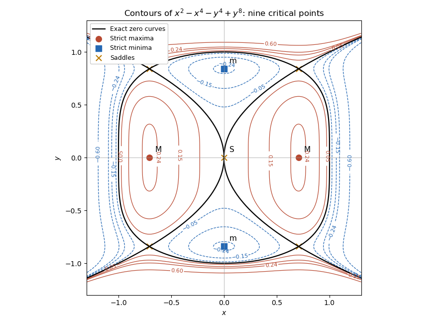
Level curves, exact zero set and all nine classified critical points of the separated quartic-octic function
. Retain the derivative marks and coefficients from the printed system. In matrix form it is , withSince , multiplication by its inverse givesThe linear transformation , diagonalizes this system:Both start at zero. An integrating factor gives , soDirect substitution into the two original equations confirms the different forcing coefficients; the exact cancellation in depends on those coefficients.
Let , with . Newton law of cooling gives the warming and cooling profilesIn the stipulated linear model, . The bacterial count obeys , so its logarithmic reduction is the cumulative thermal destruction under exponential warming and cooling:Writing , the warming integral divided by is and the cooling contribution is . Hence the required implicit equation isThe bracket is zero at zero and has derivative for , tending to infinity with . There is therefore one positive solution.
For the hardier species, is unchanged in this model if and the achieved remain the same. Raising the oven temperature changes , but its factor cancels against the changed slope of the linear destruction law. The entire normalized temperature history and hence the destruction integral remain the same; the comparison uses both the warming and equal-duration cooling stages.
The exponential distribution has survival probability for . Conditional probability therefore giveswhich proves the memoryless property. Let and . With ,The geometric distribution here starts at zero. Summing its first moment givesFor , sum the density over all integer translates:with zero density outside that interval. The integer and fractional parts of an exponential variable are independent, because for every integer and measurable ,This factorization proves independence of the discrete and continuous components, beyond just checking their separate marginals.
For the probability generating function , differentiation givesThe second derivative is a factorial moment, not the raw second moment.
In the Galton-Watson process, condition on . The next generation is a sum of independent offspring counts, and so its conditional generating function is . Averaging over givesThe conditional mean is and the conditional variance is . Thus iterated expectation gives from one ancestor, and the law of total variance gives , . Iterating yields the branching-process generation momentsFor the critical case , the correct limiting value is . If , nonnegative offspring are zero almost surely, so every later generation has zero mean and variance; handle this directly rather than use an ambiguous zero power. At generation zero the mean is one and variance zero.
The branching-process extinction criterion states that extinction probability is the smallest fixed point of in : probabilities of extinction by successive generations are the iterates of from zero, increasing to that fixed point. Here the equation is , factoring as . The two admissible roots are and one, so
Use the positive-support geometric distribution, for , . Differentiating the geometric series suppliesFor the jar, let be the waiting time to remove one red ball when exactly red balls remain. Every draw has success probability , so is geometric with that parameter. The are independent: after each success, fresh independent draws begin a new stage, and its conditional waiting distribution depends only on the deterministic count , not on earlier waiting times. Replacing a green ball leaves that stage's count unchanged.
Thus the coupon collector problem decomposition is , andThis is the coupon collector waiting-time variance. For , the formula correctly gives zero variance and a deterministic one-minute completion.
Articles were limited to the first 100 out of 215 total.
Articles by others on the same topic
There are currently no matching articles.