Original examination paper. The solutions cover all eleven questions and every requested part. The original PDF determines the parts and notation; in particular, Question 1 has a 12+8 mark allocation despite the duplicated second part and incorrect mark in the TeX transcription.
For the nonconstant boundary data, use separation of variables in polar coordinates and put . Laplace's equation reduces toThis Cauchy-Euler equation has independent solutions and . Unlike a disk containing the origin, the annulus permits both. The zero inner boundary value requires , and the outer value requires . HenceSubstituting gives zero, while gives . This is the Dirichlet problem on an annulus for one Fourier mode; no other angular mode is needed.
For the changed inner boundary value, use superposition to add a radial harmonic function that is at and zero at . The radial zero-mode equation is , giving . Imposing the two constant boundary values givesTherefore the second answer isThe logarithmic term is independent of , so it changes only the angular average of the electric potential. Both answers are unique for these Dirichlet boundary conditions, by uniqueness for Laplace's equation.
Green identity. With the outward unit normal, the product rule gives . Integrating over and applying the divergence theorem yields Green's first identity:
Uniqueness for nonzero mass. Suppose two real solutions have the same prescribed boundary data, and let be their difference. The spatial equation called the Klein-Gordon equation in the question is the modified Helmholtz equation, so . With , Green's first identity becomesFor identical Dirichlet boundary conditions, on ; for identical Neumann boundary conditions, there. Either makes the right-hand side zero. When is real and nonzero, both integrands on the left are nonnegative, forcing . ThusThis is the required uniqueness assertion; existence is understood for admissible smooth data on a suitable bounded region. Complex-valued solutions obey the same result by treating their real and imaginary parts separately.
Zero mass. For , the argument gives , hence on the connected region. Dirichlet boundary conditions still force , but Neumann boundary conditions leave an arbitrary additive constant:The prescribed normal data in the zero-mass case must also satisfy , by the divergence theorem. For nonzero , that flux can instead equal .
Energy minimization. Let for the two functions in the last part. They share their boundary values, so on . Since is a harmonic function, Green's first identity givesExpand the square in the Dirichlet energy of :The cross term vanishes, soEquality requires to be constant, and the shared boundary values then make it zero. This is the Dirichlet principle: among functions with fixed boundary values, the harmonic function minimizes Dirichlet energy.
Harmonic parts. Write the holomorphic function as . The Cauchy-Riemann equations say and . Equality of mixed partial derivatives therefore givesThus both the real and imaginary parts are harmonic functions and satisfy two-dimensional Laplace's equation.
Single-valued logarithm. A convenient choice isusing the principal logarithm for each term. Its branch cuts in the plane are and . The branch points are and : going once around the first adds , while going once around the second subtracts . Removing the two exterior rays makes this a consistent branch of a multivalued function and in particular leaves the whole open unit disk available.
Potential inside the cylinder. Put with . Multiplication by givesThe denominator is positive and the real part of the numerator is positive. Thus its argument lies strictly between and , andAs , this tends to on the upper open semicircle and on the lower open semicircle. Scale the imaginary part to obtainIt is a harmonic function, has the required boundary values, and gives . The two joining points of the boundary arcs have discontinuous boundary data, so no common continuous boundary value is demanded there. Along the real diameter, including radial approaches to either joining point, the displayed solution is zero. This is the disk potential with two semicircular boundary values.
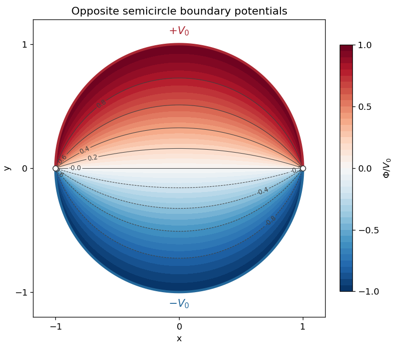

For a second check, the Taylor series of the logarithms gives . Taking the imaginary part yields the Fourier serieswhose boundary limit is exactly the required alternating pair of constant semicircle values.
Poles and residues. An isolated singularity is a pole of order if its Laurent series has finitely many negative powers, the lowest being a nonzero multiple of . The residue is the coefficient of .
If and , factor , where is holomorphic near and . For ,The last quotient is holomorphic and nonzero at , proving a simple pole with
The given function. For noninteger , specify a branch of a multivalued function before using . Choose with , a cut along the negative imaginary axis. This leaves all three roots of off the cut. They are , and , all simple. The numerator is nonzero at these points. Since the denominator has derivative , the residues areFor noninteger , zero is a branch point, rather than an isolated pole. This remains true when and the numerator diverges there. For nonnegative integer it is a regular point. Other logarithm branches change the phases of the residues consistently.
Integral and convergence. Near zero the integrand behaves as , requiring . At infinity it behaves as , requiring . Therefore the exact convergence range isUse a counterclockwise sector contour with rays at angles and , inner radius and outer radius . The same complex logarithm branch is valid throughout this sector. Only lies inside. The small circular arc contributes and the large one contributes , so both vanish precisely in the stated range.
The outward positive-real ray contributes . On the returning ray set : the denominator is still , while , with reversed limits. The residue theorem givesPut . The right-hand phase is and . HenceThe sine is positive in this range, consistent with a positive real integral. This is a special case of the Mellin integral of a reciprocal binomial.
Laplace transform. Use . The initial value is zero and the Dirac delta contributes , so the transformed equation is . Therefore
Bromwich inversion. The Bromwich inversion formula iswith the vertical Bromwich contour traversed upwards and its symmetric improper limit understood. For , close to the left, where the exponential decays; the enclosed simple pole at has residue . For , close to the right, which contains no pole. Thuswhere is the Heaviside step function. This agrees with the Laplace transform time-shift rule. At , inversion returns the average of the two one-sided values. The value assigned at that single point does not affect the differential equation in the distributional sense.
Fourier transform. State the convention explicitly:The Fourier transform of the distributional derivative is , including the jump at . The Dirac delta has transform , giving
Inverse Fourier integral. Substitute into the inverse Fourier transform:The only pole is at . For , close in the upper half-plane. Jordan's lemma removes the large arc and the residue theorem gives . For , close in the lower half-plane, where there are no poles, giving zero. This reproducesIntegrating the differential equation across the impulse checks the unit jump, . Away from the impulse the solution obeys , and it satisfies the stipulated zero past.
Tensor transformation. Under an orthogonal transformation , the magnetic moment and magnetic field intensity have transformed components , for a proper rotation. The physical relation must retain its form, giving , henceThis is precisely the law for a Cartesian second-rank tensor. Both magnetic quantities are axial vectors; under reflections they each acquire the same determinant sign, which cancels from the transformation of the magnetic susceptibility tensor.
Parallel directions. The condition is the eigenvalue equation . For the matrix in the paper, expansion of givesSolving the three resulting homogeneous systems givesThe three directions are mutually orthogonal. For the zero eigenvalue, the induced magnetic moment is zero: the proportionality equation still holds with factor zero, though there is then no nonzero moment direction to assign.
Energy extrema. The stipulated energy is . At fixed , a Lagrange multiplier calculation givesbecause is a real symmetric matrix. Thus all stationary directions are the eigenvectors, for which . Equivalently write ; thenThe Rayleigh quotient immediately givesThe intermediate direction is stationary with but is not an extremum on the sphere. At the minimum , so the precise extremum condition is proportionality, including a vanishing proportionality factor.
Constant-energy surface. In the original field components,For a fixed positive value , is unrestricted and the cross-section satisfies . The surface is therefore an elliptic cylinder, with axis along and transverse semiaxes along and along . This is an example of level sets of a positive semidefinite quadratic form. At the surface degenerates to the axis line; no negative-energy level exists.
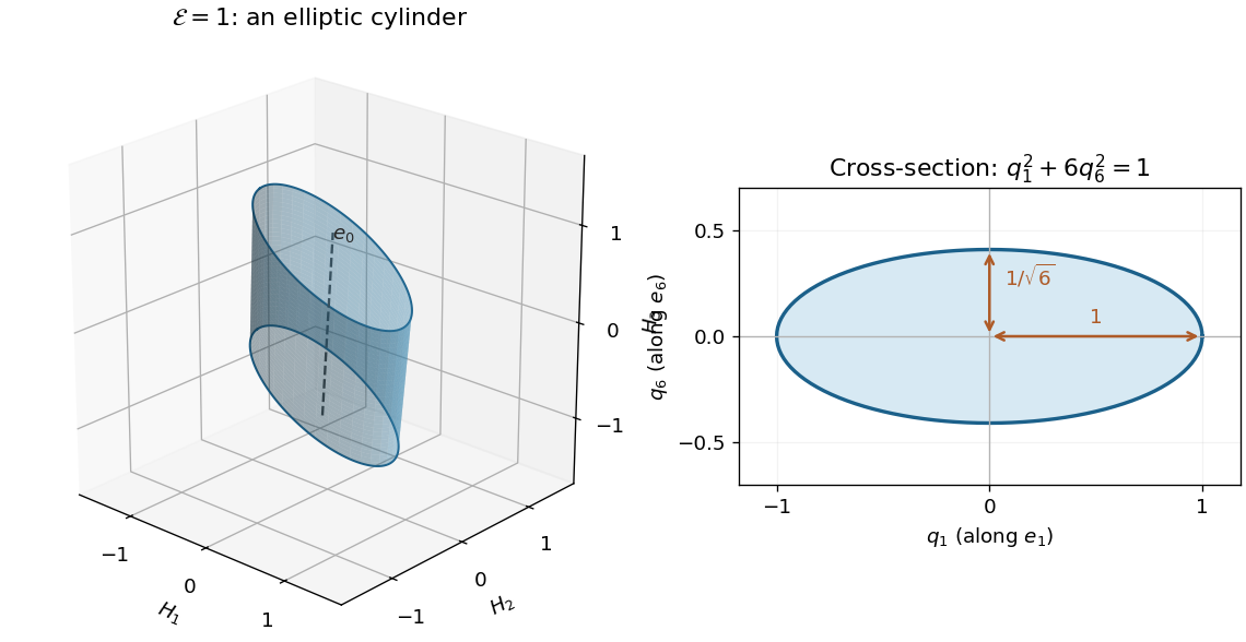
The susceptibility energy has elliptic cylindrical level sets
. The surface shown has E=1. Its unbounded axis is the zero-eigenvalue direction (1,-1,2); transverse semiaxes are 1 along e1 and 1/sqrt(6) along e6. Only a finite axial segment is drawn. Details.
General definitions. The Euler-Lagrange equation gives . Write and . A normal mode has fixed displacement pattern and common time factor, ; its normal frequency satisfiesHere is angular frequency. A normal coordinate is the coefficient of one pattern in a complete modal expansion, so these coordinates decouple the equations. Since is positive definite, the change turns the mode equation into the ordinary symmetric eigenvalue problem for .
Three-mass equations. Let be horizontal displacements from the unstretched equilibrium, ordered left to right. The kinetic energy and potential energy areDifferentiating the potential energy givesThus and
Frequencies and patterns. Put . Expansion of the generalized eigenvalue problem for small oscillations givesSolving at each root givesThe zero normal mode is uniform translation. In the lower nonzero mode, the central mass stays fixed, the two end masses move oppositely, and their unequal displacements balance both the end-mass momenta and the forces on the central mass. In the upper mode the end masses move together and the centre oppositely. Both vibrating modes leave the centre of mass fixed.
Orthogonality. Because is symmetric, two mode equations implyDistinct eigenvalues therefore give the mass-matrix orthogonality of normal modes:The Euclidean dot product need not vanish for unequal masses; for example , while . The modal squared norms are .
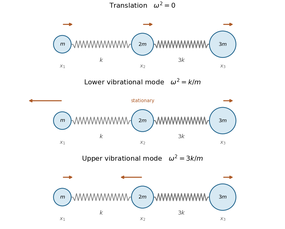

Normal coordinates. Expand . Project using the mass-weighted inner product and divide by each modal norm to obtainFor example, the inverse equations are , , . They reduce the energies toand henceThe first coordinate is the centre of mass and has free linear motion. Multiplying by respectively gives mass-normalized normal coordinates if desired.
Cosets and Lagrange. A left coset is . The left cosets of a subgroup partition a group, each with elements. Lagrange's theorem states for a finite group, so every subgroup order divides the group order.
The 64-element group. Work in the commutative ring , which has zero divisors. Denote the displayed lower triangular matrix by , where are its three entries below the diagonal. Direct matrix multiplication givesAll arithmetic is modulo four, so the set is closed. Associativity comes from matrix multiplication, the identity element is , andThe formula works in either multiplication order and requires no division. Hence these matrices form a group of order . This is the lower triangular version of the Heisenberg group over a commutative ring.
The abelian subgroup. If , write . ThenThe identity is and the inverse is , proving an abelian subgroup. Its two independent entries give and , in accordance with Lagrange's theorem. This is the abelian plane subgroup of the Heisenberg group modulo four.
More explicitly, is a surjective group homomorphism to the additive group of , with kernel . The four left cosets are exactly the four sets with fixed , ; representatives are . Thus is also a normal subgroup.
Matrices squaring to the identity. The product formula givesThe first and third coordinates vanish only when . Then modulo four, so the middle coordinate vanishes exactly when . Therefore the complete set isIt is a subgroup: multiplying two such elements keeps all three entries even, and their cross term vanishes modulo four, so the product simply adds the three even coordinates. The identity is included and each element is its own inverse. In fact is isomorphic to the direct product of groups . The seven nonidentity elements are involutions.
Finally, the last subset in the PDF is defined by , with no restriction on . It has elements, which cannot be a subgroup because does not divide . It also excludes the identity element. Thus
Definitions. A group homomorphism preserves multiplication, . A group isomorphism is a bijective group homomorphism. The kernel of a group homomorphism isPreserving multiplication implies and : the first follows by cancelling from its square, and the second follows by applying to .
Normality. For and ,Hence every is again in , proving . Applying the same statement with gives equality , and therefore .
Group of cosets. Define the product on the left cosets byTo check that this does not depend on representatives, replace by . Thenbecause normality puts in . Thus the product is well defined. It is associative because multiplication in is associative; its identity is , and the inverse of is . Consequently the cosets form the quotient group .
The map is well defined and gives an isomorphism . If the original mapping is onto , this becomes . No surjectivity is needed for the kernel of a group homomorphism to be a normal subgroup or for the quotient group to exist.
Representations. A complex group representation is a group homomorphism to the invertible linear maps on a vector space. It is an irreducible representation when and the only invariant subspaces are and .
Group table. The supplied matrices satisfy , , and . Their multiplication table isThe table proves closure and gives identity and an inverse for every element; associativity is inherited from matrix multiplication. The table is symmetric, so the group is abelian. It is the Klein four-group .
Dimensions and conjugacy. The sum of squares of irreducible representation dimensions is . A two-dimensional irreducible would alone contribute four, leaving no room for the ever-present one-dimensional trivial representation. Hence the given two-dimensional representation is reducible. Since the group is abelian, every conjugacy class is a singleton. There are therefore four inequivalent complex irreducible representations, each of dimension one:Taking the trace of the given matrices gives their character of a representation:
Irreducible characters. In a one-dimensional representation, the values on and must each be , since both elements square to . Their values determine the value on . The four choices give the complete character table:Each row is a character because it respects the generating relations, and the rows have unit norm and pairwise zero character inner product. The multiplicities of these rows in are respectively , by character orthogonality. Thus
Diagonal form. The common invariant lines are spanned by and . Use their normalized vectors as columns ofThen simultaneous diagonalization givesReading the first and second diagonal entries across the four matrices recovers and , respectively, verifying the decomposition explicitly.
Fourth-order spatial formula. For a sufficiently smooth function, pair the Taylor expansions at opposite shifts:Multiply the first sum by sixteen, subtract the second, and subtract . The constant and fourth-derivative terms cancel, leavingHence the fourth-order centered second derivative satisfiesRearranging proves the requested , including its leading error coefficient.
Explicit diffusion scheme. Take , , , and let approximate . Combining the forward Euler method in time with in space givesTo check the error, insert the exact solution. The heat equation gives , while the time Taylor expansion and the spatial formula give the one-step defectThus its unnormalized local truncation error isas requested. Dividing this defect by gives the normalized residual ; these are distinct error conventions.
Boundary implementation. The centered stencil requires two ghost values at each end. An even-reflection closure for Neumann diffusion imposesThe reflected first centered difference at either endpoint is zero. Apply the same evolution formula at the endpoints after substituting these ghost values; for example,The ghost values also close the stencil at and . They are determined auxiliary values, not new physical data. For a smooth solution compatible with the Neumann boundary conditions, differentiating those conditions in time and using the heat equation gives at the endpoints. Thus even reflection preserves the smoothness needed for fourth-order spatial accuracy. If the initial data fail the required higher compatibility conditions, a uniform smooth error expansion through cannot be assumed.
For completeness, the reflected spatial operator has cosine eigenvectors and eigenvaluesThe most negative one is . Requiring gives the forward Euler method stability restriction in the natural trapezoid-weighted discrete norm. A fourth-order spatial stencil does not remove the explicit diffusion time-step restriction.
Implicit alternative. The Crank-Nicolson diffusion scheme using the same spatial operator and boundary closure isIt has second-order time accuracy and fourth-order spatial accuracy for smooth compatible solutions; its one-step defect is . Each spatial eigenvalue has amplification factor of magnitude at most one, so it removes the explicit restriction for this boundary closure.
The price is solving a banded linear system at every step; the same matrix factorization can be reused for fixed and . Large time steps still reduce accuracy. Moreover, the amplification factor tends to as , so short spatial wavelengths can alternate sign with little numerical damping. Thus unconditional linear stability does not guarantee a monotone or well-resolved transient. Boundary accuracy and initial compatibility remain necessary with either time discretization.
Articles by others on the same topic
There are currently no matching articles.