For the weighted inner product, the factor cancels the in the Sturm-Liouville operator. Assuming the coefficients are real, two applications of integration by parts giveThis is the boundary form in the Lagrange identity for a Sturm-Liouville operator. The potential terms cancel; if were complex, an additional integral of would remain, so suitable real coefficients are part of formal self-adjointness. The endpoint restrictions in part (a) eliminate the displayed form for every pair of functions in the domain.
The necessary boundary identity for a self-adjoint operator isAt regular endpoints, a standard full family of separated self-adjoint conditions iswith real coefficients and neither pair , zero. For example, if , both functions obey at , so there. The cases and the endpoint follow directly. These include Dirichlet boundary conditions, Neumann boundary conditions and Robin boundary conditions.
Separate vanishing at each endpoint is sufficient but not necessary. Coupled conditions such as and , with real , make the two endpoint forms equal and hence their difference zero. More generally the allowed endpoint data must be a maximal subspace on which the boundary form vanishes; this ensures that the adjoint has the same domain. Merely imposing extra endpoint restrictions until the boundary term vanishes proves symmetry, but can overrestrict the domain and fail to give self-adjointness.
Let . By self-adjointness,Taking first shows that each eigenvalue is real: for a nonzero eigenfunction, since . ThereforeFor distinct eigenvalues this proves orthogonality of Sturm-Liouville eigenfunctions:The weight is essential: this need not be orthogonality under the unweighted integral.
The useful coordinate for this scale-dependent differential operator is . With , the chain rule givesThe interval becomes , and the endpoint values become . This logarithmic change of variable in a Sturm-Liouville problem reduces the calculation to a constant-coefficient Dirichlet problem. Also , so the transformation preserves the appropriate weighted inner product.
Divide the eigenvalue equation by and collect the first two derivative terms into a single derivative:Thus one choice of Sturm-Liouville form isIndeed . Both and are positive and regular throughout this interval. The zero endpoint values make the boundary form vanish.
In logarithmic coordinates the eigenvalue problem becomes . A nonzero function with zero values at both ends requires : multiplying by and integrating gives . Write . The first endpoint gives , and the second requires , .
For vector normalization, . A positive real normalization constant therefore givesThe sine orthogonality identity also gives . Completeness is the usual completeness of the Fourier sine series on under the logarithmic coordinate transformation.
Expand the forcing and the solution in the normalized eigenfunctions: and . Their coefficients areSince all are nonzero, the equation gives . Hence the required Sturm-Liouville eigenfunction expansion isThis is constant forcing in a logarithmic Dirichlet Sturm-Liouville problem. The coefficients are , so the solution series converges uniformly and has zero endpoint values. Applying is justified in the weighted square-integrable sense; the forcing sine series equals one at interior points, while its endpoint sums are zero. The equation is imposed in the interior, so this does not contradict the boundary conditions.
As an independent check, solving directly givesIt has both zero endpoint values and satisfies . The invertibility of the Dirichlet operator makes it the same solution as the expansion.
Use separation of variables, writing . After multiplication by , the radial and angular terms are functions of independent variables, so setWith , the angular equation isRegularity at both poles selects , , and the Legendre polynomials ; the other angular branch is singular at a pole. The radial Euler-Cauchy equation is . A power gives , hence .
Superposing these axisymmetric spherical harmonics givesThe coefficients must give convergence appropriate to the domain. In a region containing the origin, regularity removes the negative powers; in an exterior region with zero potential at infinity, it removes the growing powers and the constant. No such radial restriction is needed for a general annular region.
Resolve the angular surface charge density into Legendre polynomials:For a single degree , write the common surface potential as . Regularity and decay require radial factors inside and outside. Their exterior-minus-interior radial derivative at is . Thus spherical harmonic matching with a derivative jump gives .
Only degrees zero and two occur, yieldingBoth expressions have surface value , and their derivative difference is , checking both interface conditions. The interior quadratic is regular at the origin, and the exterior potential tends to zero.
The leading far-field term is the monopole term. Indeed the total charge is , and the normalization of the specified jump gives . No extra permittivity factor is inserted into the supplied normalization. Regularity here means finite piecewise smooth potential; its normal derivative necessarily jumps at the charged surface.
For the vector field , the product rule givesThe mixed dot products cancel. The divergence theorem therefore yields Green's second identity,The fields and boundary are assumed sufficiently regular. A singular Green function can be treated by excising a small ball around its source and taking the radius to zero, or using distributions.
Fix the evaluation point inside and put in Green's second identity. The two terms cancel because and . The remaining volume integral is . ThusThe Dirac delta has a positive sign in this problem's Green-function equation, fixing the order of the two terms. All boundary derivatives act on the integration variable .
Impose a homogeneous Dirichlet boundary condition on the Green function in its first variable, for . The second boundary term then vanishes, givingIn a bounded domain, a Dirichlet Green function requires not to be a Dirichlet eigenvalue of ; otherwise a resonance can obstruct its existence. The representation assumes such a Green function exists.
In all space, put and try . For , direct differentiation gives , so the Helmholtz equation holds away from the source. Integrate its inhomogeneous version over a small source-centred ball. The volume integral tends to zero, while the flux isIt must equal the integrated delta, one. ThereforeThis is the negative of the convention used in the outgoing Green function for the three-dimensional Helmholtz equation, where the source is . The sign here follows the present convention. The factor chooses the outgoing solution, with time convention and the Sommerfeld radiation condition; one could add homogeneous solutions without a radiation prescription.
Reflect to . The method of images gives the Dirichlet image kernel for the three-dimensional Helmholtz equation:The two distances coincide on the plane, so its boundary value is zero; the image source is outside the domain. It therefore has the required positive delta source inside and the selected outgoing behaviour.
Let . At a boundary point , the distances to the real and reflected sources have derivatives and . ThusThe outward unit normal of the upper half-space is , and . HenceUsing the decay assumption to discard the distant hemisphere in the boundary representation givesThe qualification at infinity concerns the whole Green boundary term, not just the pointwise limit of . Sufficient decay of the field and its derivatives, as assumed, makes it vanish; compatible radiation conditions can also do so. As a sign check, taking in the kernel gives , the positive Poisson kernel for the upper half-space.
Put . The two roots areSince , their moduli are and . Thus exactly one root is inside the unit circle, and neither lies on it.
For the real integral use , so and . The change of variables givesThe contour is counterclockwise. At its single interior simple pole, the residue isBy the residue theorem, the reciprocal affine sine integral is thereforeThe condition also makes the real denominator strictly positive, consistent with the positive answer and the absence of contour poles on the unit circle.
Use the principal branch of the complex logarithm for . Its branch cut is the ray , , lying below the real axis. Thus it is analytic in the upper half-plane, where the only pole of the integrand is .
Close the real interval by a large upper semicircle. The estimation lemma bounds the arc integral by , so it vanishes. The simple-pole residue isThe residue theorem then givesFor real , . Taking real parts and then using evenness of the real integrand yieldsBoth endpoints converge: the integrand is near zero and at infinity. This also agrees with the logarithmic parameter integral with Cauchy weight at parameter one.
The Fourier transform of is : two integrations by parts have no boundary terms under the stated decay assumption. Time differentiation commutes with the spatial transform. ThereforeFor every fixed spatial wavenumber , this is a constant-coefficient ordinary differential equation in time.
The characteristic polynomial is , with roots . For , the transformed general solution isThe repeated-root case is , rather than two independent copies of the same exponential. An alternative basis regular at is , using the limit for the last factor at zero.
For , the Fourier shift theorem turns the two exponential factors into translations. Equivalently, set ; then . The D'Alembert formula gives the general formwhere are arbitrary functions with the required regularity and decay. The arbitrary profiles can accommodate a spatially transformed zero-frequency velocity by their integral components; the isolated repeated root must not be used to discard that degree of freedom. If , the equation instead has .
This is the exponentially conjugated wave equation. Positive produces damping, but the algebra also covers negative , which gives exponential amplification. The sign of is immaterial because the differential equation contains only .
The initial profile is , with the absolute value confirmed in the original PDF. Its Fourier transform isUsing in the regular cosine-sine form giveswith the quotient interpreted as when . Put . Inverting, or applying the D'Alembert formula to , whose initial velocity is , givesFor an explicit expression at , let and . The integral is for and for . ThereforeThe branches agree at . At zero time, the integral vanishes and the translated profiles coincide, recovering . Their time derivatives cancel, while the integral contributes , cancelling the derivative of the prefactor, so .
For the limiting answer is . The cusp in means the solution is understood as a weak solution, classically smooth away from the characteristic fronts ; it is not globally twice differentiable. No assumption that is positive is needed for this initial-value solution.
For a constant orthogonal Cartesian change of coordinates , the tensor component transformation law for order isRepeated indices are summed. In Cartesian orthonormal coordinates the metric identifies upper and lower indices, so the same orthogonal matrix acts on every index.
An isotropic tensor has the same numerical components after every proper orthogonal change of axes: for every with and . For example, is isotropic because . Some conventions require invariance under all orthogonal transformations, including reflections; this stronger convention must be distinguished for odd-order tensors, notably the Levi-Civita symbol, which is invariant under proper rotations but changes sign under its ordinary three-index transformation for a reflection.
Under the same Cartesian change, a vector field has with . The chain rule gives . Since is constant,This is exactly the order-two tensor component transformation law. Thus the Cartesian vector gradient is a Cartesian second-rank tensor, as in the velocity gradient tensor when is a velocity field.
The restriction to Cartesian transformations matters. In a general position-dependent basis, differentiating the basis contributes extra terms, so the tensorial derivative is the covariant derivative, not an arbitrary array of partial derivatives.
An axial vector transforms under an orthogonal matrix asFor a proper rotation, , so this is the usual polar vector rule. Under an orientation-reversing change, the extra sign distinguishes the two. In particular, spatial inversion leaves an axial vector unchanged while reversing a polar vector.
Let . The determinant identity for the Levi-Civita symbol isIt follows by multiplying the three-index determinant identity by and using orthogonality. The derivative transformation from part (ii) then givesHence the curl of a polar vector field is an axial vector field. The Levi-Civita determinant factor is exactly the extra sign required under reflections.
Write . The trace fixes the isotropic part, and splitting the remaining matrix into its symmetric and antisymmetric parts gives the scalar, symmetric-traceless and axial tensor decomposition:Here and . The antisymmetric part is . Its associated axial vector isIndeed the contraction identity gives . Adding the three parts reconstructs .
The minus sign is required by the index order . The symmetric gradient and curl decomposition written instead for has the opposite axial sign. The divergence supplies , the trace-free symmetric part describes shape change, and the antisymmetric part describes local rotation.
Direct differentiation givesThe curl is , so the preceding convention givesPut . The normalized principal axes and eigenvalues of the symmetric tensor areThe planar axes lie along the two angle bisectors of the coordinate axes. If , one planar direction extends and the perpendicular direction contracts, with no change along the third axis. The labels need not be ordered by size when . If , then , all principal values vanish and any orthonormal frame is a principal frame; the flow is pure local rotation in the plane.
The kinetic energy is . Differentiating the quadratic potential energy gives the equations for small oscillations,Put and . The eigenvalue problem is . Its characteristic polynomial isThus a convenient set of normal modes isEach shape can be multiplied by an arbitrary sinusoidal time amplitude. In the lowest mode all beads move in phase. In the middle mode the central bead is fixed and the outer beads move oppositely. In the highest mode the two outer beads move together against the centre. These vectors are mutually orthogonal and span the three displacement coordinates.
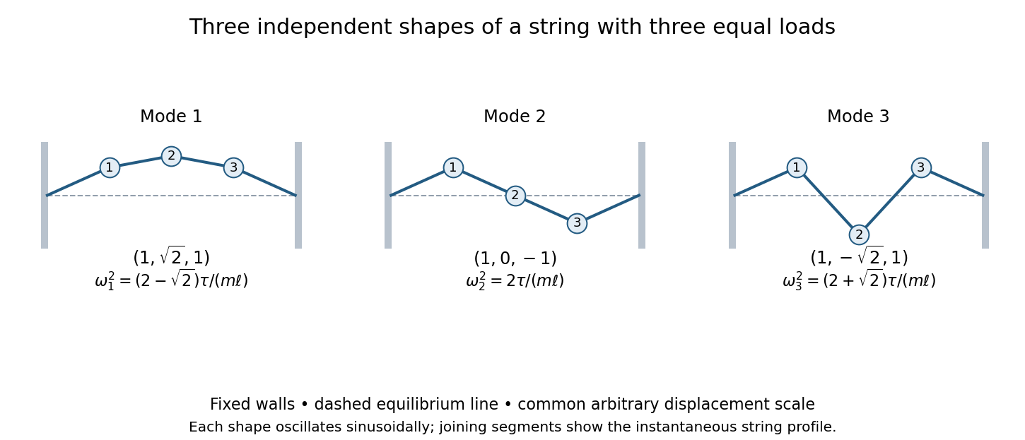
The three transverse string modes; the dashed line is equilibrium and bead displacements share one arbitrary scale
. Details. 
These are the three-mass case of the normal modes of a uniformly loaded finite string, with discrete sine shapes . The sketches use straight string segments between masses and fixed zero displacements at the walls. The small-slope and constant-tension assumptions justify the quadratic energy and linear equations.
Resolve the initial displacement into the mode shapes from part (i):There is no component along : the initial displacement is invariant under exchanging beads 1 and 3, whereas that mode is antisymmetric. Zero initial velocities select cosine time dependence. ThereforeHere and . At zero time these expressions give and all three velocities vanish.
The motion is a superposition of the two symmetric normal modes, with opposite signed modal amplitudes. The outer beads always move together. Equivalently, , displaying the modulation from the two frequencies. The result describes the linearized string while the initial amplitude and subsequent slopes remain small compared with the bead spacing.
The identity commutes with every group element, so it lies in the center of a group. If are central and , then implies . ConsequentlyThus is central. The subgroup test provesEquivalently, the centre is nonempty, closed under products, and closed under inverses. This proof does not require finiteness. In fact the centre is an Abelian subgroup, and it is normal because for each central element.
Write the cyclic factors additively. The order of a group element in a direct product of groups is the least common multiple of its component orders, since a power is the identity exactly when it is the identity in both coordinates.
In , has order , so it generates all six pairs. An explicit group isomorphism isIt is well defined and multiplicative in additive notation; its kernel is zero because an integer divisible by both two and three is divisible by six. Equal finite orders then give bijectivity.
In , every element has order dividing four. A generator of has order eight, and isomorphisms preserve element orders, soFor positive integers , the maximum element order in is , attained by a pair of generators. The product is cyclic of order exactly when that number is . Thus cyclicity of a product of two finite cyclic groups givesFor coprime factors the map gives the isomorphism, the group form of the Chinese remainder theorem.
For a subgroup of a finite group , Lagrange's theorem statesHere is the number of distinct left cosets. Every coset has members, and the cosets partition , proving the identity. In particular the order of a subgroup divides the order of the group. Divisibility is generally necessary, not sufficient, for a subgroup of a given order to exist.
The relation implies . Move each reflection generator to the right in any word, cancel pairs using , and reduce exponents modulo . Every element then has a normal form or , .
For the actual symmetry group of a regular polygon these are distinct rotations and distinct reflections. The determinant distinguishes rotations from reflections in the planar action. Hence the source's dihedral group has order , with its subscript counting polygon vertices. The calculations below use that convention.
For a regular pentagon, take as rotation through and as reflection in the horizontal axis through vertex zero. The distinct elements areEvery nonidentity rotation has order five. The reflections are the five order-two elements, since .
The reflection has axis at angle to the horizontal, understood modulo . If vertices have angles , it sends vertex to vertex . Each axis passes through one vertex and the midpoint of the opposite edge; that vertex stays fixed and the other four vertices exchange in two pairs.
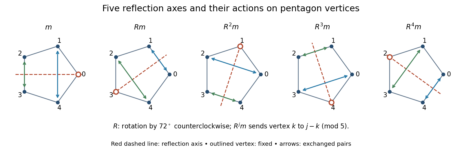
The five order-two pentagon symmetries; each dashed reflection axis fixes one vertex and exchanges the two indicated pairs
. Details. 
Since , Lagrange's theorem permits proper subgroup orders only . The complete list isTo show completeness, an order-two subgroup must be generated by its unique nonidentity element, necessarily one of the five reflections. An order-five subgroup is cyclic, since its order is prime; its generator cannot be a reflection, and every nonidentity rotation generates the same rotation subgroup. There is only one order-one subgroup.
Thus there are seven proper subgroups when the trivial subgroup is included, or six nontrivial proper subgroups. These are the prime-sided case of the classification of subgroups of a dihedral group.
The conjugacy class of is . Rotations commute with one another, while conjugation by a reflection changes to . Thus the rotation classes are , and .
For reflections,Because multiplication by two permutes the residues modulo five, these conjugates exhaust all five reflections. Consequently the complete class partition isTheir sizes account for every element, as in the conjugacy classes of a finite dihedral group.
A normal subgroup is a union of complete conjugacy classes. The trivial subgroup is normal, and the rotation subgroup is normal because conjugation preserves it; equivalently it has index two. None of the five order-two subgroups is normal, because it contains just one member of the five-element reflection class. Thus the proper normal subgroups are exactly
A group representation assigns each an invertible linear map on a fixed vector space, preserving multiplication:Choosing a basis turns those maps into matrices. A faithful representation is injective, equivalently its kernel is , so distinct elements have distinct matrices.
Two group representations on spaces of the same dimension are called equivalent representations if one fixed invertible change of basis conjugates every representing matrix: for all . Choosing a different separately for each element does not establish equivalence.
The character of a representation isThe cyclic property of the trace makes it invariant under a change of basis and constant on conjugacy classes. Thus different characters at even one group element prove inequivalence.
Since , multiplication adds exponents modulo four: . Hence the Cayley table of the cyclic group of order four, with the left factor indexing rows, isThe table is symmetric because the group is Abelian. Its row for each element permutes all four members, as cancellation requires.
The matrices are listed in the order . In the first representation, is the clockwise quarter-turn matrix and . In the second, , whose successive powers give the listed scalar matrices. Both therefore obey the group table and distinguish all four elements.
Taking traces gives the characters of a representation:In particular but . Since trace is invariant under similarity, the representations are inequivalent, even after allowing complex changes of basis for the real matrices of .
One can also see the obstruction directly: conjugating the scalar matrix leaves it unchanged, whereas is not scalar. Over the complex numbers, has eigenvalues , while has ; those different multiplicities cannot be removed by changing basis.
Write the lower block of as . ThenA representation of must satisfy its defining relation , so . For real , this means or ; it also ensures invertibility.
If , then while . The image of the generator has order four, so its four powers are distinct and the representation is faithful. If , then but , since the lower block has zero diagonal. The image has order two and the kernel is . HenceFor other values there is no representation of , rather than an additional unfaithful case; in particular would make the assigned matrix singular. These conclusions are the faithfulness criterion for a block representation of the cyclic group of order four. There is no requirement that the proposed representation be orthogonal, so no separate conditions should be imposed.
Articles by others on the same topic
There are currently no matching articles.