Past exam of the physics A course of the University of Cambridge / 2018 / Paper 1 / Section B

Let $\rho ={\psi }^{\ast }\psi$ be the probability density. For a real potential energy $V(x)$, the Schrödinger equation and its complex conjugate areDifferentiate $\rho$ and substitute both equations. The potential terms cancel, leavingComparison with the probability continuity equation ${\partial }_t\rho +{\partial }_{x}J=0$ identifiesFor a plane wave of amplitude $A$ and positive wavenumber $k$, $J=\hslash k|A{|}^2/m$, the density times the velocity. Integrating the continuity equation over an interval makes its probability change equal to the incoming current minus the outgoing current.

SetAll are real and $k_0>k_1>k_2>0$. Suppressing a common time quantum phase $e^{-iEt/\hslash }$, chooseThe rightmost region has no left-moving term because no wave is incident from the right. The shifted quantum phase convention makes $F$ the transmitted amplitude at the second interface.

For finite potential steps and equal mass, wavefunction matching at a finite potential step requires continuity of both $\psi$ and ${\partial }_x\psi$. Explicitly,A discontinuous wavefunction would introduce an inadmissible singular kinetic term, while integrating the stationary Schrödinger equation across a finite step shows that the derivative cannot jump. These conditions also keep the probability current continuous, so a finite interface neither creates nor destroys probability. The derivative rule would need modification for a delta-function potential or a different effective mass; neither occurs here.

Zero reflection means $B=0$. Matching the first interface then givesThe specified layer quantum phase is $k_{1}a=\pi /2$, so $e^{i{k}_{1}a}=i$ and $e^{-i{k}_{1}a}=-i$. The second-interface conditions becomeSince $C+D=A$, compatibility requires $\boxed{k_1^2=k_0{k}_2}$. This is a quantum quarter-wave matching layer: the intermediate wavenumber is the geometric mean, and the two interface reflections cancel after their round trip through the layer.

In terms of the physical energies,Rearranging also givesA finite positive energy satisfying the stated ordering requires $V_2/2<V_1<V_2$. Under that condition $E-V_2=(V_2-V_1{)}^2/(2V_1-V_2)>0$, consistent with the assumed propagating transmitted wave. The width must simultaneously satisfy the given quarter-wave quantum phase condition.

From the second-edge amplitude in part (c),This uses ${\psi }_{\mathrm{R}}=F{e}^{i{k}_2(x-a)}$. If the transmitted wave is instead written $T{e}^{i{k}_{2}x}$, its coefficient is $\boxed{T/A=i\sqrt{k_0/k_2}{e}^{-i{k}_{2}a}}$; the extra factor only changes the quantum phase convention.

Using the probability current of a plane wave,Thus the flux transmission probability is one. The larger transmitted density $|F{|}^2>|A{|}^2$ compensates for the smaller transmitted velocity $\hslash k_2/m$; equal currents need not have equal wave amplitudes.

The one-dimensional time-independent Schrödinger equation isHere $m$ is the particle mass, $V(x)$ its potential energy, $E$ the stationary energy eigenvalue, and $\hslash =h/(2\pi )$ the reduced Planck constant. The spatial wavefunction is $\Psi$; the full stationary state is $\Psi (x)e^{-iEt/\hslash }$. Physical bound states satisfy the boundary conditions and wavefunction normalization $\int |\Psi {|}^{2}dx=1$. The operator on the left is the Hamiltonian operator, the sum of kinetic and potential energies.

Assume $a>0$ and define $\omega =\sqrt{2a/m}$ so that the potential is that of a quantum harmonic oscillator. The two trial forms have derivativesSubstitution into the stationary Schrödinger equation cancels the $x^2$ terms precisely when $a=2{\hslash }^2{C}^2/m$. Normalizability selects the positive root,The remaining constants giveFor later overlaps choose positive normalization constants. The Gaussian integral gives $A=(2C/\pi {)}^{1/4}$, while its second-moment integral gives $B=2\sqrt{C}A$. Thus both wavefunctions have unit norm and are orthogonal by their opposite parity.

The real Gaussian is positive everywhere and has no nodes; the odd state has exactly one node at $x=0$. The Sturm oscillation theorem orders one-dimensional bound states by their node count. Consequently these are the ground state and first excited state, respectively, also agreeing with the oscillator spectrum $E_n=(n+1/2)\hslash \omega$.

The infinite wall imposes $\boxed{\Psi (0)=0}$, and the wavefunction vanishes for $x<0$. The even full-oscillator ground state fails this boundary condition; the lowest admissible state is the positive-half restriction of the odd first excited state. Multiplying by $\sqrt{2}$ restores normalization because half its probability originally lay on either side.

With $\ell =\sqrt{\hslash /(m\omega )}$, the half-harmonic oscillator ground state isIt rises from zero at the wall, reaches its wave-amplitude maximum at $x=\ell$, and decays to zero as $x\to \infty$. It is positive throughout the interior of the allowed region, with no interior node, as required for its ground state. The wall need not make the derivative continuous with the forbidden half-line.

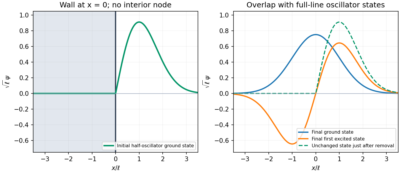
For removal of a half-oscillator wall, the sudden approximation keeps the state unchanged during the change of potential. Its probability in the new full-oscillator ground state ${\Psi }_0={\pi }^{-1/4}{\ell }^{-1/2}{e}^{-x^2/(2{\ell }^2)}$ is the squared overlap:where ${\int }_0^{\infty }x{e}^{-x^2/{\ell }^2}dx={\ell }^2/2$. ThereforeThe integral runs only over the initially occupied half-line. The initial state is not the odd full-line eigenstate: it is zero, rather than negative, on the left. Indeed its overlap with that final first excited state is $1/\sqrt{2}$, giving probability $1/2$, and the remaining probability lies in higher states. Subsequent evolution under the new fixed Hamiltonian operator changes the quantum phases of its energy components without changing these energy-measurement probabilities.

The quantum rotor has orientation angle $\varphi$ of period $2\pi$, so physical wavefunctions satisfy $\psi (\varphi +2\pi )=\psi (\varphi )$. The exponential solutions of $Hu=Eu$ are thereforeThey are normalized and orthogonal on $[0,2\pi )$. The corresponding angular momentum operator is $L_z=-i\hslash {\partial }_{\varphi }$, with eigenvalue $m\hslash$. The $m=0$ ground level is nondegenerate, and every $|m|>0$ energy level has the twofold degeneracy $m\leftrightarrow -m$. This uses ordinary periodic boundary conditions, with no flux or twisted quantum phase.

Expand the initial wavefunction in the angular momentum eigenbasis using ${\cos }^2\varphi =1/2+(e^{2i\varphi }+e^{-2i\varphi })/4$. With the normalized $u_m$ from part (a), this givesThe coefficient squares sum to one, also verifying the stated normalization. The Born rule therefore gives angular momentum outcomesFor an energy measurement the two distinct $m=\pm 2$ states belong to the same energy eigenspace. Sum their probabilities, rather than adding their amplitudes, to obtainTheir relative probabilities are $4:1:1$ for the angular momenta and $2:1$ for the energies. In particular, zero mean angular momentum does not imply zero rotational energy.

Each energy eigenstate evolves by its own quantum phase $e^{-i{E}_{m}t/\hslash }$. The two $m=\pm 2$ components have the same energy, while the $m=0$ quantum phase stays one. ThusIn angle representation this isAt $t=0$, $1+\cos 2\varphi =2{\cos }^2\varphi$ recovers the initial state. The fixed coefficient magnitudes keep the angular momentum and energy probabilities constant even though the density in angle changes.

Taking the modulus squared gives the three-mode revival of a planar quantum rotor:The angular density has period $\pi$, while both the state and its density revive after $\boxed{T=2\pi /\Omega =\pi I/\hslash }$. Its integral over $0\le \varphi <2\pi$ is one because $\int \cos 2\varphi d\varphi =0$ and $\int {\cos }^{2}2\varphi d\varphi =\pi$.

At $t=0$, the density is $4{\cos }^4\varphi /(3\pi )$, with maxima at $0,\pi$ and zeros at $\pi /2,3\pi /2$. At $t=T/2$ it becomes $4{\sin }^4\varphi /(3\pi )$, interchanging those maxima and zeros. At $t=T/4$ and $3T/4$, it is $[1+{\cos }^{2}2\varphi ]/(3\pi )$, with four equal maxima along the coordinate axes and positive minima halfway between them. At $t=T$ the original profile returns.

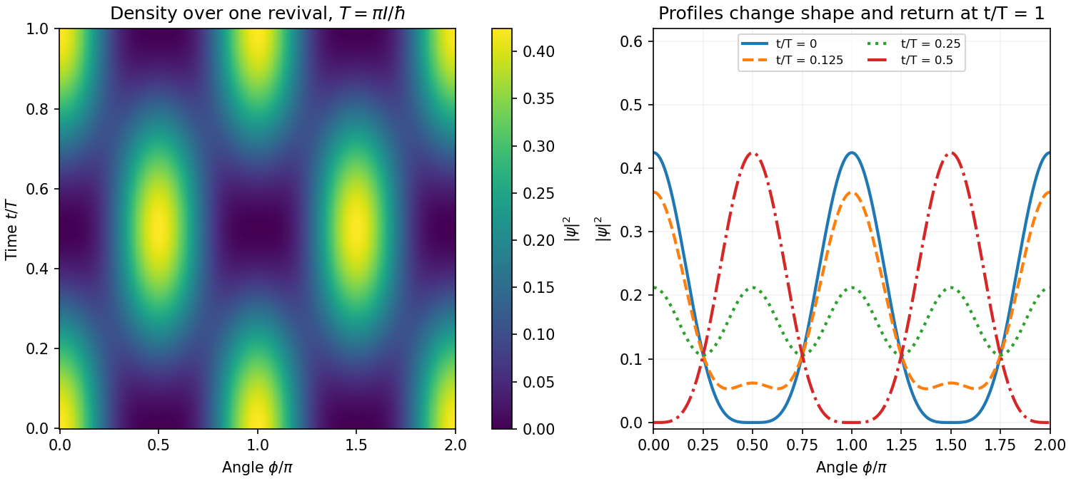
The changing profile is interference between the stationary $m=0$ mode and the degenerate counter-rotating $m=\pm 2$ modes. It does not translate rigidly around the circle; the standing-wave weights alternate between two orientations.

The commutator is $\boxed{[A,B]=AB-BA}$. To evaluate it for differential operators, apply it to a smooth test wavefunction $f$:Thus the canonical commutation relation is $\boxed{[x,p_x]=i\hslash I}$. The associated Heisenberg uncertainty relation is $\Delta x\Delta p_x\ge \hslash /2$. Position and momentum cannot both have arbitrarily sharp outcome distributions in the same prepared state, even with ideal measuring apparatus. This concerns quantum-state preparation, not merely a calibration error in a particular instrument.

Expand the proposed product rule without interchanging any operator factors:Applying this commutator identity with $A=x$ and $B=C=p_x$ givesFor a differentiable multiplication potential, apply the other commutator to a test function:ThereforeThese operator equalities are understood on a common domain where the indicated products and derivatives are defined, with the boundary conditions appropriate to the state.

For a normalized state, the expectation value isFor a time-independent operator, differentiation givesThe Schrödinger equation says $|\dot{\psi }⟩=-iH|\psi ⟩/\hslash$. The self-adjointness of $H$ gives $⟨\dot{\psi }|=i⟨\psi |H/\hslash$, soIn the integral derivation, the same self-adjointness step is integration by parts with vanishing boundary terms. An explicitly time-dependent observable would also contribute $⟨\partial Q/\partial t⟩$. These are the expectation-value equations underlying the Heisenberg equation of motion.

The Hamiltonian operator isSince multiplication by $x$ commutes with multiplication by $V(x)$, part (b) gives $[x,H]=i\hslash p_x/m$. Similarly $[p_x,H]=-i\hslash V^{\prime }(x)$. Substituting into part (c) gives Ehrenfest theorem:Thus the mean momentum changes according to the mean force, and the derivative of mean position is mean velocity. These exact quantum equations resemble Hamilton's classical equations, but $⟨V^{\prime }(x)⟩$ generally differs from $V^{\prime }(⟨x⟩)$. The classical point-particle equation for the center is exact for potentials at most quadratic and is an approximation for a localized packet when the force varies little across it. A spatially broad packet in a nonlinear potential need not follow a classical trajectory. Even where its center follows classical motion, its width and measurement uncertainties remain quantum properties.