Changing basis and acceleration. Attach orthonormal unit vectors to the rotating frame, with a common origin fixed in the inertial frame. An infinitesimal rotation changes a vector fixed in those axes by : its tip moves tangentially to the circle about the rotation axis. More generally, write . Differentiating the components and the rotating basis separately proves the rotating-frame derivative formula,
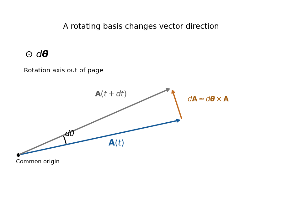
Original geometric construction of the tangential change of a vector during a small positive rotation; the change is dtheta crossed with A
. Details. 
Apply the formula first to position: , where . Apply it again to both terms. For constant ,One cross term comes from differentiating in the inertial frame and another from differentiating in . The displayed source formula implicitly requires constant angular velocity and an unaccelerated common origin. For changing rotation rate there is also ; an accelerating origin supplies its own translational acceleration. Moving the rotation terms to the force side gives the apparent Coriolis force and centrifugal force with negative signs.
Southward motion on Earth. Use local east, north and up axes, with latitude positive northward. Then and . The Coriolis acceleration in local Earth coordinates givesIt is westward in the northern hemisphere, eastward in the southern hemisphere and zero for exactly southward motion at the equator. There is no vertical Coriolis component for this particular velocity.
Correct steering. On the desired meridional track, drag has no eastward component because it is antiparallel to the velocity. If the thrust makes signed angle east of south, its eastward component is . The cross-track force balance is thereforesoThe argument must have magnitude at most one for this simple thrust-only correction to be feasible. The signed angle changes sign at the equator: correction is east of south in the north and west of south in the south. Thus the phrase “east of south” cannot describe a positive correction throughout the entire flight.
Wrong-sign correction and the miss distance. A literally constant velocity vector cannot develop a cross-track displacement. The physically useful interpretation of the last task is constant speed, with an erroneous lateral steering correction. In the usual leading-track model, thrust and drag balance along the actual motion, and the applied transverse correction has the correct magnitude but the wrong sign. It therefore reinforces rather than cancels the Coriolis force. Starting at the equator, use the unperturbed southward track , and let be the eastward departure from that track. To first order in the departure,There is a factor two relative to uncompensated Coriolis deflection because the wrong correction adds an equal lateral force. Integration gives the wrong-sign Coriolis steering error,For southern angular distance , and , the nominal flight time after the equator isTaking givesThe small-latitude approximation gives and , or , confirming the scale and direction.
This is an estimate under an explicit steering model, not an exact trajectory forced by the wording. For example, retaining spherical transport of the local axes while still linearizing in the cross-track motion gives, with , . Consequently and the longitude departure is . The distance along the destination parallel is then . Corrections from the changed track and a more detailed control law are not fixed by the problem. If “keeps the velocity constant” instead means the full vector, the pilot would need an additional compensating force and there would be no miss; if thrust is kept at a specified geographical bearing despite drift, its along-track component and lateral drag must also be modelled.
Radial energy and effective potential. For a central force with potential energy , angular momentum conservation fixes and confines motion to a plane. The kinetic energy separates into radial and angular parts, givingThe second term is the centrifugal barrier. It converts the radial motion to a one-dimensional energy problem: allowed radii have , turning points have equality, and a circular orbit occurs at a stationary point of . Stability of that radial orbit requires a local minimum.
The first-order orbit equation. Write . Since , choose zero potential at infinity to getAlso . Substitute this into the energy equation and multiply by :Here has units of length. A regular bound orbit with a centrifugal barrier requires as well as the appropriate negative energy.
Solving in inverse radius. Let and defineDividing the first-order equation by givesDifferentiating, or directly using the Binet equation, gives . The continuation through turning points follows from this smooth second-order equation. Its noncircular bound solution, with angular origin at a pericentre, isSubstitution into the first-order equation fixes the amplitude through this . Therefore the requested representation holds withsince . A general angular origin replaces by . This is the orbit equation for combined inverse-square and inverse-cube attraction. The circular limit is regular in but is not represented by finite in the source's normalized cosine form.
Precession and the inferred length. The last expression immediately givesSuccessive pericentres occur after angular advance , so the apsidal precession per orbit isFor near one, . Inferring an inverse-cube perturbation from apsidal precession consequently gives . For the stipulated nearly circular approximation, , and Kepler's third law givesusing , and . A century contains about orbits. Convert the observed advance to radians per orbit before using it:HenceThe positive sign strengthens the attraction and gives prograde precession. The fractional perturbation validates the small-deviation expansion. This is the parameter fitting the proposed phenomenological force law under the specified small-eccentricity approximation, not a derivation of that law as the physical explanation of Mercury's anomaly.
Normal-mode idea. Near a stable equilibrium, expand the potential energy to quadratic order and the kinetic energy as a quadratic form in generalized velocities. The Euler-Lagrange equations then take the linear form . A normal mode has fixed displacement ratios, , with . Real systems admit this description for sufficiently small motion, before higher-order nonlinearities or strong damping matter. Superposition permits a general motion to be assembled from the modes. A free symmetry direction may instead be a zero mode, with constant or linearly changing coordinate.
Lagrangian and bead equations. Take each as an arc-length displacement positive in the same sense around the fixed circular wire. Spring length changes are , and . Equal equilibrium spring tensions give no net tangential force; their linear energy terms sum to zero. Dropping an irrelevant constant, the Lagrangian isFor example, differentiating the potential with respect to gives . The three Euler-Lagrange equations therefore areThe wire supplies normal constraint forces but does no tangential work. These are the equal-mass case of the normal modes of three beads connected by springs on a circular hoop.
Frequencies. The stiffness matrix divided by isIt annihilates . On the two-dimensional subspace , its action is multiplication by three. Thus the angular frequencies of the normal modes areThe repeated frequency is a degeneracy of normal modes, while the zero frequency expresses free rigid rotation of all beads along the wire.
General solution. Two independent vectors spanning the vibrating subspace are and . Each amplitude satisfies , with . The uniform coordinate satisfies . HenceThe six freely specifiable real constants give the six initial data; is fixed by and is not an additional independent integration constant. The linear zero-mode term must be included to allow nonzero total tangential momentum.
Shapes and uniqueness. In the first term beads 1 and 2 have opposite equal displacements and bead 3 remains at its equilibrium position. In the second term beads 1 and 3 do this while bead 2 stays fixed. The last term moves all three identically, leaving spring extensions unchanged: is a rigid phase shift and a uniform drift around the wire. The sketches show positive modal amplitudes; all arrows reverse half a vibration period later.
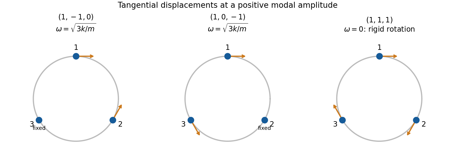
Original displacement sketches for two independent equal-frequency bead modes and the rigid-rotation zero mode; arrows indicate displacement along the ring rather than its radius
. Details. 
The two nonzero-frequency eigenvectors are not unique, because any independent linear combinations in their degenerate two-dimensional eigenspace form an equally valid basis. In particular the displayed pair is independent but not orthogonal; one could use and instead. The zero eigenspace is one-dimensional, so its vector is fixed up to scale and sign.
Specified release. Zero initial velocities permit and require . At , the three displacement conditions become , , . Therefore one convenient set of constants isEquivalently,Their sum remains , as required by zero initial total tangential momentum. Alternative amplitude signs with compensating phase shifts represent the same motion.
Constitutive law and Poisson ratio. Use positive stress for tension. In an isotropic linearly elastic medium, Hooke's law givesThe analogous equations follow by cyclic permutation. Under uniaxial tension in direction 1, and . Thus Poisson's ratio measures transverse contraction relative to longitudinal extension when the transverse stresses are zero. It is dimensionless; it is not the ratio of transverse stress to longitudinal stress.
Radial and hoop strains. Let a material point originally at radius move to , with small axisymmetric displacement. Two neighbouring radii separated by move apart by , so the radial fractional extension is . A circle's circumference changes from to , so its fractional extension is . ConsequentlyThe absence of longitudinal stress is a plane stress condition, not a claim of zero longitudinal strain.
Equilibrium of an annular wedge. Consider a slice of unit axial length, radial thickness and small angular width . The difference of the outward and inward radial face forces is to leading order. The two tangential face tensions have inward radial resultant : each contributes . With no body force, their balance gives the radial equilibrium of a thick elastic cylinder,This hoop contribution is why the radial stress need not be spatially constant in a thick wall.
Displacement equation. With , the two Hooke's law equations readInvert them:Substitute in . After cancelling the common factor, the right-hand side is , soThe cancellation explains why this displacement equation does not depend on the value of Poisson's ratio.
Power laws and wall pressure. Try . The indicial equation is , soThe resulting Lamé stress distribution in a pressurized cylindrical wall can be writtenThe pressure boundary tractions are and . Solving them yieldsHence the positive compressive radial pressure in the wall isIt equals at and at . This directional radial pressure is not an isotropic fluid pressure: radial and tangential stresses differ. The associated displacement is . Also , generally nonzero even though .
Maximum absolute tangential stress. For , and . Therefore the maximum of its absolute value must be at one of the two surfaces. Keeping the specified external pressure gives the fully general answerFor the usual high internal pressure with negligible external pressure, the largest magnitude is the tensile stress on the inner wall:For finite , the inner-wall expression is , but its absolute value is not always the larger endpoint value. For example, nearly equal internal and external pressures can leave the outer surface more compressive. With , both stresses correctly reduce to everywhere. These results use a homogeneous linear elastic wall without axial loading; a closed-ended pipe would require a different longitudinal-stress condition.
Articles by others on the same topic
There are currently no matching articles.