Selected final answers: Partial answer sheet, PDF page 175. This sheet does not cover every question.
Write the plate area as and separation as , so the original capacitance is . Neglect edge fields. The greatest capacitance occurs when each material occupies half the plate area and spans the full separation. These two regions are capacitors in parallel, sharing the same electric potential difference:The least capacitance occurs when a dielectric layer of thickness covers the whole area, leaving a vacuum layer of the same thickness. The two layers are capacitors in series: the normal electric displacement field is continuous and the voltage drops add. Their individual capacitances are and , givingThe arithmetic-harmonic bounds for dielectric capacitance show that these are genuine extrema over other arrangements of the same two volumes, within the ideal parallel-plate model. A uniform trial electric field in the fixed-voltage energy principle bounds above by the arithmetic mean of the two permittivities; a uniform trial electric displacement field in the fixed-charge principle bounds it below by their harmonic mean. The two layer arrangements attain those bounds. Both reduce to when .
In steady rigid rotation of the liquid about its vertical axis, centrifugal acceleration is outward. Hydrostatic pressure balance in the rotating frame givesThe free surface is at constant atmospheric pressure, so its slope obeysCompare this parabolic free surface of a rigidly rotating liquid with . For focal length ,Either sense of rotation gives the same shape. The result assumes the liquid has reached rigid rotation before solidifying and that surface-tension and solidification distortions can be neglected.
Use , to recognize the planar quadrupole potential, . Its electric field is minus the gradient:or, in cylindrical coordinates,For , arrows point toward the origin along the axis and away from it along the axis. The off-axis electric field lines satisfyThe axes themselves are the separating field lines; the origin is a field null. Reversing reverses every arrow. The field is independent of , and has units .
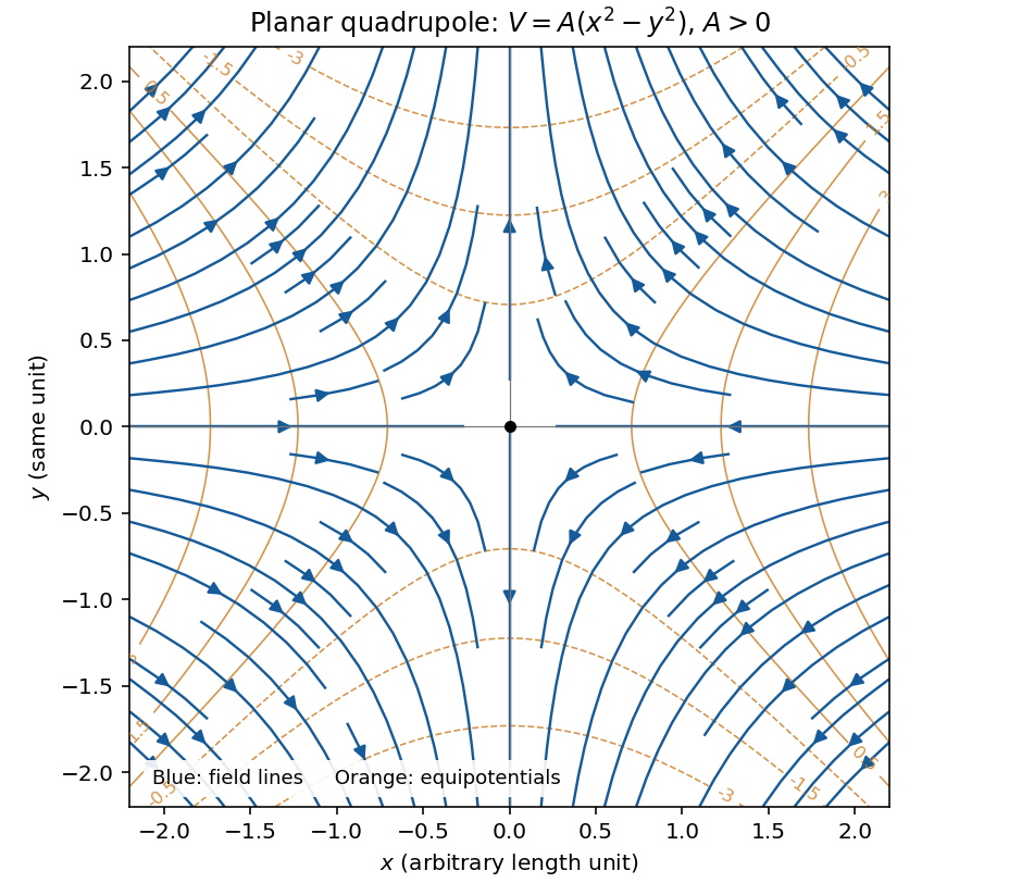
Original calculated electric-field lines and equipotentials for the planar quadrupole with positive A; arrows approach along x and leave along y
. Details. 
First estimate the excess pressure as weight divided by contact area:For the equilibrium estimate, use the Clapeyron equation for melting. The specific volume change on melting is , and the latent heat of fusion gives . Thus the common-pressure melting-point slope isTake and the usual rounded water density , in addition to the supplied and . ThensoThe sign is negative because ice contracts on melting. This is a linear equilibrium estimate treating the load as a common local pressure on coexisting ice and water. The actual contact stress is nonuniform, and frictional heating, deformation and drainage also affect skating; the estimate is not a complete account of the lubricating water film.
Cold air is denser than room air at approximately the same pressure. The ideal gas law gives a fractional mass density contrast of order . The initial outflow is therefore a gravity current driven by reduced gravityFor an illustrative refrigerator height , room temperature and temperature difference , this gives . Balancing the released potential energy with kinetic energy gives . The buoyancy exchange time of a cold-air enclosure is consequentlyUsing constant acceleration over height gives , consistent at this level. Warm air enters as cold air leaves, so unrestricted vacuum free fall is not the right acceleration model. No dimensions or temperatures are specified in the source, so an order-of-magnitude estimate with explicit representative values is the appropriate result; shelves and mixing can delay complete replacement.
Images and uniqueness. The method of images replaces a conducting boundary by fictitious charges outside the physical field region. Choose them so that the resulting electric potential satisfies the required conductor potentials. The Uniqueness of the Dirichlet problem then guarantees the same physical exterior field. For example, a point charge at height above a grounded plane has an image at height : the plane is an equipotential at zero, and the charge is attracted toward it by . The image is a computational device; the physical conductor carries a continuous induced surface charge density.
Potential of a line. Surround an infinite line charge by a coaxial Gaussian cylinder of radius and length . Gauss's law gives , hence . Integrating givesWriting an additive constant instead is equivalent. The reference length makes the logarithm dimensionless; an isolated infinite line cannot be assigned a finite zero potential at infinity.
Locating the two lines. Put the grounded plane at and the physical cylinder at , with axis along and radius . Set , and place line charges and at and . If and are their distances from an observation point, the cylinder-plane image charges giveOn , , so . To check the cylinder, define . The level set is a circle: completing the square givesSince , its centre is and radius is . The positive line lies inside the cylinder; the negative line lies behind the plane. There is consequently no fictitious charge in the exterior physical region. A Gaussian contour around the cylinder encloses only, so the required physical charge per unit length is also correct. These boundary conditions and the far-field behaviour determine the physical solution by Uniqueness of the Dirichlet problem.
Cylinder voltage. The constant distance ratio on the cylinder immediately givesIts capacitance per unit length is . In the thin-cable limit, .
Cable attraction. Because the cable is idealized as infinite, the meaningful answer is force per unit length. For , centre height and ,The electrostatic attraction per unit length of a cylinder above a plane isFor example, this follows without any ambiguity about moving image positions from at fixed voltage, including the work of the voltage source. Its sign is negative because capacitance decreases with height. A cable length experiences approximately downward when end effects are negligible. This is the electrostatic contribution only.
Inductance and interface conditions. For a linear coil, self-inductance is the ratio of its own magnetic flux linkage to current. Its induced electromotive force is for fixed . Across an interface with unit normal from medium 1 to 2,These electromagnetic boundary conditions follow from Gauss's law for magnetism and Ampère's law. Here is free surface current. At the iron–air faces there is no free surface current, so normal magnetic flux density and tangential magnetic field intensity are continuous. In each isotropic linear medium, .
Complete core. A slender toroid has approximately uniform along mean path length . Ampère's law gives , so . The flux per turn is , yielding the inductance of a toroidal winding,This uses constant relative magnetic permeability and neglects leakage, fringing and saturation.
Why the gap lowers inductance. The gap replaces an easy magnetic path in iron with air. Maintaining the same flux now requires a much larger magnetic field intensity in part of the path and therefore more ampere-turns. Equivalently, magnetic reluctance increases, so the flux linkage for a fixed current and hence self-inductance decrease. A narrow gap can matter greatly because its permeability is smaller by the factor .
Oblique-gap calculation. In the original diagram is the perpendicular separation of the cut faces. Let point along the core, and let be normal and tangential to the gap faces. With the face at angle to the core direction, . Write the core flux density as . The boundary conditions givesoThe gap area normal to its nearly normal field is , not . Its leading reluctance is consequently . Adding the core reluctance gives the inductance of a toroid with an oblique narrow air gap,Thus at ,The approximation retains the possibly order-one ratio while neglecting , fringing and the small tangential gap contribution. More precisely, a local uniform-field path along the core, with missing iron length subtracted, gives denominator . Its correction is beyond the stipulated large-, narrow-gap accuracy; simply neglecting would not be justified.
Field in the slot. The component expression above givesFor the gap and ,Its units are . The field is almost perpendicular to the cut faces, rather than following the iron direction straight across the cut. Its small angle away from the face normal satisfies at ; the sense reverses if the current reverses.
Field law and centre value. The Biot-Savart law for a steady thin wire isHere follows the conventional electric current and the displacement points from source to observation point. For a circular loop of radius , every element at the centre has distance and contributes in the same axial direction. Choose by the right-hand rule. Then
On-axis integration. At axial distance , every wire element has distance . Azimuthal symmetry cancels transverse components. Parameterizing gives axial cross-product element , so the on-axis magnetic field of a circular current loop isIt points the same way on the two halves of the axis; its strength is even in .
Directions near the axial point. At a point on the positive axis the field is axial, but nearby lines spread outward because decreases as increases. On the negative-axis side they converge toward the axis while still progressing in the positive axial direction. There is no azimuthal field. The near-axis sketch shows this local spreading; the complete magnetic field lines return around the outside of the loop and form closed curves.
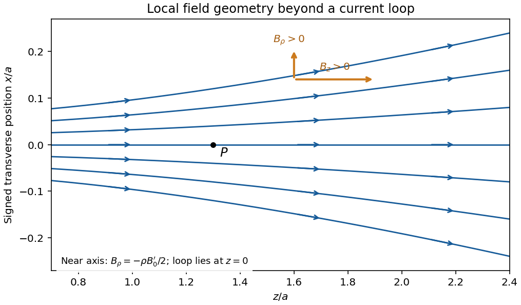
Original calculated leading near-axis field-line geometry on the positive side of a circular current loop; the lines spread as the axial field weakens
. Details. 
Radial component from zero divergence. Smooth axial symmetry gives and . By Gauss's law for magnetism,Integrate radially from zero, excluding a singular term, to obtain the near-axis radial magnetic field, . Differentiating the axial field therefore givesFor it is outward; for it is inward. This supplies the direction reasoning used in the sketch.
Force on the second loop. Put the second loop at and radius . For , the radial field due to the first loop is . The element experiences Lorentz forceThe radial contributions cancel as vectors around the loop. The axial contributions add, giving the force between distant coaxial current loops,The sign follows . Both the small radial coordinate relative to and the dipole approximation are justified by .
Force direction. The second loop is pulled back toward the first: the force is attractive for the same current sense. Reversing one current reverses the force. The much larger axial field chiefly produces radial element forces; retaining the smaller radial field is essential for the net axial attraction.
Field equations. In a homogeneous source-free nonmagnetic medium, and . Maxwell's equations becomeThe first equation follows from for spatially constant nonzero . When the effective relative permittivity is negative below, its charge response is already included in ; it must not also be counted as an extra free source.
Amplitude relations and bulk dispersion. Work with complex phasors proportional to . For , the Ampere-Maxwell law givesso the amplitudes must obeyThey are not arbitrary independent constants: the dispersion relation alone would not make arbitrary amplitudes satisfy the equations. These relations give , so the electric divergence vanishes; the magnetic divergence vanishes because there is no dependence. The only nonzero component of Faraday's law of induction isSubstitution then givesThis proves that all four field equations hold for the specified transverse magnetic polarization when both the amplitude relations and the dispersion relation are imposed.
Interface matching. Let region 1 be vacuum above the interface, with , ; region 2 has , . These signs make the evanescent fields decay as . In the absence of free surface current, tangential is continuous, giving a common interface amplitude. Tangential is also continuous, henceNormal is continuous as well: both sides have . This does not require itself to be continuous; the material can have polarization surface charge. The normal magnetic field is zero on both sides.
Existence and surface dispersion. The opposite signs of and require . The two bulk equations areUse to eliminate the decay constants. For the nontrivial interface branch,A positive together with real propagating gives . A negative permittivity between and zero is insufficient. This lossless planar surface-plasmon dispersion describes a surface plasmon polariton; would instead be identical media and supplies no decaying bound mode.
Frequency range and long wavelengths. With , the existence condition becomesThe upper value is a limiting frequency approached as , not an attained maximum at finite . Substitution into the dispersion relation givesFor , choosing propagation in the positive direction,It approaches the vacuum light line from larger . The vacuum decay constant is then , so confinement becomes weak at low frequency. This calculation assumes the stated real, lossless effective permittivity; dissipation would require complex propagation and decay constants.
Changing basis and acceleration. Attach orthonormal unit vectors to the rotating frame, with a common origin fixed in the inertial frame. An infinitesimal rotation changes a vector fixed in those axes by : its tip moves tangentially to the circle about the rotation axis. More generally, write . Differentiating the components and the rotating basis separately proves the rotating-frame derivative formula,
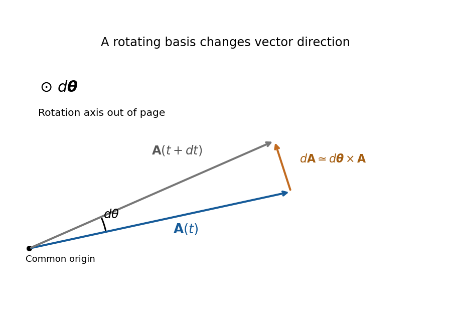
Original geometric construction of the tangential change of a vector during a small positive rotation; the change is dtheta crossed with A
. Details. 
Apply the formula first to position: , where . Apply it again to both terms. For constant ,One cross term comes from differentiating in the inertial frame and another from differentiating in . The displayed source formula implicitly requires constant angular velocity and an unaccelerated common origin. For changing rotation rate there is also ; an accelerating origin supplies its own translational acceleration. Moving the rotation terms to the force side gives the apparent Coriolis force and centrifugal force with negative signs.
Southward motion on Earth. Use local east, north and up axes, with latitude positive northward. Then and . The Coriolis acceleration in local Earth coordinates givesIt is westward in the northern hemisphere, eastward in the southern hemisphere and zero for exactly southward motion at the equator. There is no vertical Coriolis component for this particular velocity.
Correct steering. On the desired meridional track, drag has no eastward component because it is antiparallel to the velocity. If the thrust makes signed angle east of south, its eastward component is . The cross-track force balance is thereforesoThe argument must have magnitude at most one for this simple thrust-only correction to be feasible. The signed angle changes sign at the equator: correction is east of south in the north and west of south in the south. Thus the phrase “east of south” cannot describe a positive correction throughout the entire flight.
Wrong-sign correction and the miss distance. A literally constant velocity vector cannot develop a cross-track displacement. The physically useful interpretation of the last task is constant speed, with an erroneous lateral steering correction. In the usual leading-track model, thrust and drag balance along the actual motion, and the applied transverse correction has the correct magnitude but the wrong sign. It therefore reinforces rather than cancels the Coriolis force. Starting at the equator, use the unperturbed southward track , and let be the eastward departure from that track. To first order in the departure,There is a factor two relative to uncompensated Coriolis deflection because the wrong correction adds an equal lateral force. Integration gives the wrong-sign Coriolis steering error,For southern angular distance , and , the nominal flight time after the equator isTaking givesThe small-latitude approximation gives and , or , confirming the scale and direction.
This is an estimate under an explicit steering model, not an exact trajectory forced by the wording. For example, retaining spherical transport of the local axes while still linearizing in the cross-track motion gives, with , . Consequently and the longitude departure is . The distance along the destination parallel is then . Corrections from the changed track and a more detailed control law are not fixed by the problem. If “keeps the velocity constant” instead means the full vector, the pilot would need an additional compensating force and there would be no miss; if thrust is kept at a specified geographical bearing despite drift, its along-track component and lateral drag must also be modelled.
Radial energy and effective potential. For a central force with potential energy , angular momentum conservation fixes and confines motion to a plane. The kinetic energy separates into radial and angular parts, givingThe second term is the centrifugal barrier. It converts the radial motion to a one-dimensional energy problem: allowed radii have , turning points have equality, and a circular orbit occurs at a stationary point of . Stability of that radial orbit requires a local minimum.
The first-order orbit equation. Write . Since , choose zero potential at infinity to getAlso . Substitute this into the energy equation and multiply by :Here has units of length. A regular bound orbit with a centrifugal barrier requires as well as the appropriate negative energy.
Solving in inverse radius. Let and defineDividing the first-order equation by givesDifferentiating, or directly using the Binet equation, gives . The continuation through turning points follows from this smooth second-order equation. Its noncircular bound solution, with angular origin at a pericentre, isSubstitution into the first-order equation fixes the amplitude through this . Therefore the requested representation holds withsince . A general angular origin replaces by . This is the orbit equation for combined inverse-square and inverse-cube attraction. The circular limit is regular in but is not represented by finite in the source's normalized cosine form.
Precession and the inferred length. The last expression immediately givesSuccessive pericentres occur after angular advance , so the apsidal precession per orbit isFor near one, . Inferring an inverse-cube perturbation from apsidal precession consequently gives . For the stipulated nearly circular approximation, , and Kepler's third law givesusing , and . A century contains about orbits. Convert the observed advance to radians per orbit before using it:HenceThe positive sign strengthens the attraction and gives prograde precession. The fractional perturbation validates the small-deviation expansion. This is the parameter fitting the proposed phenomenological force law under the specified small-eccentricity approximation, not a derivation of that law as the physical explanation of Mercury's anomaly.
Normal-mode idea. Near a stable equilibrium, expand the potential energy to quadratic order and the kinetic energy as a quadratic form in generalized velocities. The Euler-Lagrange equations then take the linear form . A normal mode has fixed displacement ratios, , with . Real systems admit this description for sufficiently small motion, before higher-order nonlinearities or strong damping matter. Superposition permits a general motion to be assembled from the modes. A free symmetry direction may instead be a zero mode, with constant or linearly changing coordinate.
Lagrangian and bead equations. Take each as an arc-length displacement positive in the same sense around the fixed circular wire. Spring length changes are , and . Equal equilibrium spring tensions give no net tangential force; their linear energy terms sum to zero. Dropping an irrelevant constant, the Lagrangian isFor example, differentiating the potential with respect to gives . The three Euler-Lagrange equations therefore areThe wire supplies normal constraint forces but does no tangential work. These are the equal-mass case of the normal modes of three beads connected by springs on a circular hoop.
Frequencies. The stiffness matrix divided by isIt annihilates . On the two-dimensional subspace , its action is multiplication by three. Thus the angular frequencies of the normal modes areThe repeated frequency is a degeneracy of normal modes, while the zero frequency expresses free rigid rotation of all beads along the wire.
General solution. Two independent vectors spanning the vibrating subspace are and . Each amplitude satisfies , with . The uniform coordinate satisfies . HenceThe six freely specifiable real constants give the six initial data; is fixed by and is not an additional independent integration constant. The linear zero-mode term must be included to allow nonzero total tangential momentum.
Shapes and uniqueness. In the first term beads 1 and 2 have opposite equal displacements and bead 3 remains at its equilibrium position. In the second term beads 1 and 3 do this while bead 2 stays fixed. The last term moves all three identically, leaving spring extensions unchanged: is a rigid phase shift and a uniform drift around the wire. The sketches show positive modal amplitudes; all arrows reverse half a vibration period later.
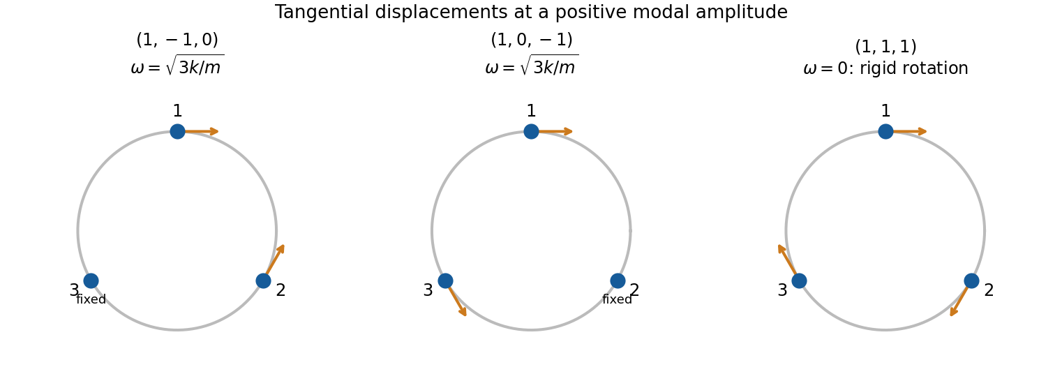
Original displacement sketches for two independent equal-frequency bead modes and the rigid-rotation zero mode; arrows indicate displacement along the ring rather than its radius
. Details. 
The two nonzero-frequency eigenvectors are not unique, because any independent linear combinations in their degenerate two-dimensional eigenspace form an equally valid basis. In particular the displayed pair is independent but not orthogonal; one could use and instead. The zero eigenspace is one-dimensional, so its vector is fixed up to scale and sign.
Specified release. Zero initial velocities permit and require . At , the three displacement conditions become , , . Therefore one convenient set of constants isEquivalently,Their sum remains , as required by zero initial total tangential momentum. Alternative amplitude signs with compensating phase shifts represent the same motion.
Constitutive law and Poisson ratio. Use positive stress for tension. In an isotropic linearly elastic medium, Hooke's law givesThe analogous equations follow by cyclic permutation. Under uniaxial tension in direction 1, and . Thus Poisson's ratio measures transverse contraction relative to longitudinal extension when the transverse stresses are zero. It is dimensionless; it is not the ratio of transverse stress to longitudinal stress.
Radial and hoop strains. Let a material point originally at radius move to , with small axisymmetric displacement. Two neighbouring radii separated by move apart by , so the radial fractional extension is . A circle's circumference changes from to , so its fractional extension is . ConsequentlyThe absence of longitudinal stress is a plane stress condition, not a claim of zero longitudinal strain.
Equilibrium of an annular wedge. Consider a slice of unit axial length, radial thickness and small angular width . The difference of the outward and inward radial face forces is to leading order. The two tangential face tensions have inward radial resultant : each contributes . With no body force, their balance gives the radial equilibrium of a thick elastic cylinder,This hoop contribution is why the radial stress need not be spatially constant in a thick wall.
Displacement equation. With , the two Hooke's law equations readInvert them:Substitute in . After cancelling the common factor, the right-hand side is , soThe cancellation explains why this displacement equation does not depend on the value of Poisson's ratio.
Power laws and wall pressure. Try . The indicial equation is , soThe resulting Lamé stress distribution in a pressurized cylindrical wall can be writtenThe pressure boundary tractions are and . Solving them yieldsHence the positive compressive radial pressure in the wall isIt equals at and at . This directional radial pressure is not an isotropic fluid pressure: radial and tangential stresses differ. The associated displacement is . Also , generally nonzero even though .
Maximum absolute tangential stress. For , and . Therefore the maximum of its absolute value must be at one of the two surfaces. Keeping the specified external pressure gives the fully general answerFor the usual high internal pressure with negligible external pressure, the largest magnitude is the tensile stress on the inner wall:For finite , the inner-wall expression is , but its absolute value is not always the larger endpoint value. For example, nearly equal internal and external pressures can leave the outer surface more compressive. With , both stresses correctly reduce to everywhere. These results use a homogeneous linear elastic wall without axial loading; a closed-ended pipe would require a different longitudinal-stress condition.
Articles by others on the same topic
There are currently no matching articles.