Source release: www.whatdotheyknow.com/request/earth_science_past_papers_and_ex/response/3419815/attach/4/Papers.zip?cookie_passthrough=1
A useful idealization is a thin sedimentary cover over a felsic upper continental crust, an intermediate middle continental crust, and a more mafic lower continental crust, ending at the Mohorovičić discontinuity at about 35–40 km. The boundaries within the continental crust are approximate compositional divisions, not three universal sharp interfaces.
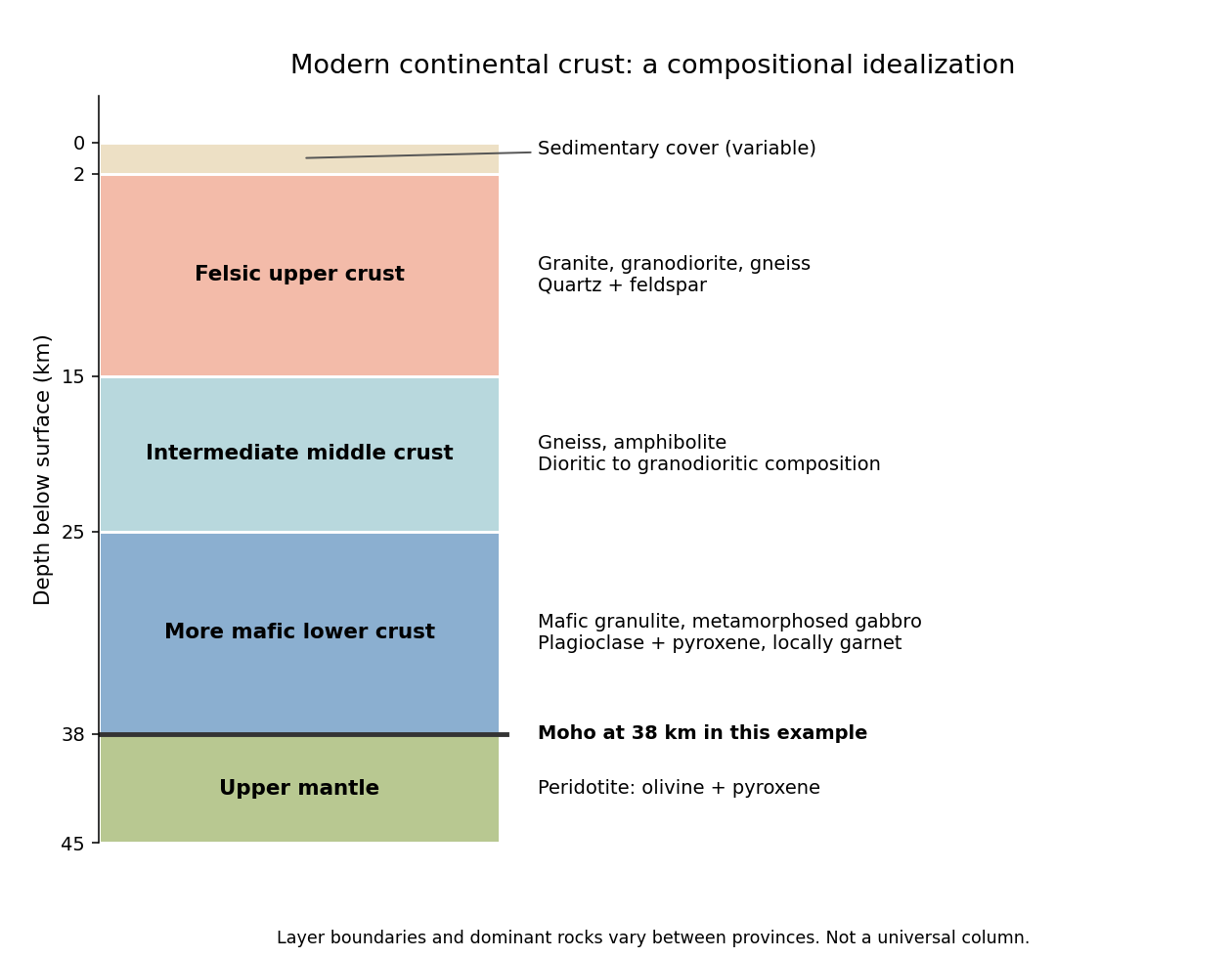
An idealized modern continental crustal column
. An original schematic for a 38 km thick continental crust. Depth ranges illustrate a compositional tendency; individual provinces have different lithologies and boundaries. Details.
- At the surface, a variable, commonly kilometre-scale sedimentary cover contains sediments and sedimentary rocks. Exposed crystalline basement can instead occur at the surface.
- In the upper roughly 15 km, representative rocks are granite, granodiorite and compositionally related gneiss, with quartz and feldspar. Sedimentary rocks, metamorphic rocks and volcanic rocks make this layer heterogeneous.
- At roughly 15–25 km, intermediate gneiss and amphibolite-facies assemblages become important. Diorite to granodiorite compositions and amphibole- and plagioclase-bearing rocks are representative.
- At roughly 25–38 km, mafic granulite and gabbro-derived metamorphic rocks are a useful average, with plagioclase, pyroxene and sometimes garnet. Some provinces instead have substantially intermediate or felsic lower continental crust.
- Below the Mohorovičić discontinuity is peridotite of the mantle, dominated by olivine and pyroxene. This is not a fourth crustal layer.
The important trend is increasing average mafic character with depth, rather than a change from granite directly to peridotite. Granulite describes a metamorphic facies, not a unique chemical composition. The synthesis in Nature and composition of the continental crust: A lower crustal perspective by Roberta L. Rudnick and David M. Fountain combines seismic and petrological evidence for these distinctions.
The expected broad contrast is a less mature, commonly thinner early juvenile continental crust, with more mafic material and abundant sodic tonalite-trondhjemite-granodiorite, rather than the more differentiated, potassium-rich granitoid component characteristic of much Phanerozoic continental crust. This is a secular tendency, not a single stratified column applicable throughout the Archean.
Archean terrains commonly expose tonalite-trondhjemite-granodiorite gneiss associated with greenstone belts containing basalt, komatiite and metasedimentary rocks. Many later granitoids are richer in potassium, including granite and granodiorite. The proportions changed during the Archean: a reconstruction from trace element ratios in sedimentary rocks infers a markedly mafic upper continental crust before about 3.0 Ga and a more felsic upper continental crust by 2.5 Ga. Thus “all Archean continental crust was mafic” would be wrong. A preserved tonalite-trondhjemite-granodiorite-dominated nucleus can be strongly felsic, including at depth; its composition is not identical to that of its original juvenile precursor.[ref]
Thickness needs a stated comparison. An influential seismic compilation found preserved Archean crust about 27–40 km thick, commonly without the thick high-velocity basal layer of its 40–55 km thick Proterozoic comparison provinces. That supports a relatively thin endmember, but is not a measurement of every original Archean continental crust, nor a demonstration that every Archean region was thinner than today's 35–40 km reference column. Tectonic thickening, magmatic underplating, erosion, delamination and preservation bias all alter what survives. The very thick lithospheric mantle beneath a craton must also not be mistaken for thick continental crust.[ref]
The transferable answer is therefore more mafic early juvenile precursors, widespread sodic tonalite-trondhjemite-granodiorite production, and variable thickness evolving through time; late Archean felsic nuclei can already resemble substantial modern continental crust.
Today the usual first melt is basaltic melt from the mantle wedge; in a hotter Archean subduction zone, melting of hydrated basaltic crust itself could generate sodic felsic melt of tonalite-trondhjemite-granodiorite composition. Distinguish a primary melt from the evolved melt ultimately added to the upper continental crust.
On the modern Phanerozoic Earth:
- Hydrothermal alteration introduces water into the incoming oceanic crust and locally into serpentinized mantle. Sediments also carry water in pore space and hydrous minerals.
- As the slab descends, heating and metamorphism break down hydrous minerals. Released fluids enter the hotter peridotite of the mantle wedge and lower its solidus, causing flux melting. Most ordinary modern slabs release fluids before extensive melting of their basaltic crust.
- The primary melt is predominantly hydrous basaltic magma. During ascent, storage and fractional crystallization, mafic minerals are removed and the remaining liquid evolves toward andesite, dacite and rhyolite compositions. Partial melting of recently emplaced mafic lower continental crust, magma mixing and some crustal contamination can contribute to felsic magma. Intrusive equivalents include diorite, tonalite and granodiorite.
This adds juvenile material derived from the mantle; simply remelting old continental crust is reworking, not net juvenile addition. The amount and depth of slab water release depend on its thermal history, as quantified in Subduction factory: 4. Depth-dependent flux of H2O from subducting slabs worldwide by Peter E. van Keken and others.
For the hotter Archean endmember posited in the question, a hotter mantle and a warm descending plate make it easier for hydrated basaltic crust to reach its solidus. Its partial melting can directly make silica-rich, sodium-rich tonalite-trondhjemite-granodiorite liquids, leaving a more mafic residue. Residual garnet and amphibole, and the presence or absence of residual plagioclase, help determine the rare-earth element and strontium signatures. These are not ultramafic liquids merely because the surrounding mantle was hotter.
The contrast is therefore commonly fluid-fluxed mantle melting followed by differentiation today, versus a greater potential contribution from direct melting of hydrated mafic crust in the hotter case. Tonalite-trondhjemite-granodiorite is not unique evidence for subduction: melting of thickened mafic crust can produce similar liquids. Nor are all modern arcs devoid of slab melting. These qualifications are central to The composite Archaean grey gneisses: Petrological significance, and evidence for a non-unique tectonic setting for Archaean crustal growth by Jean-François Moyen.
Hotter Archean mantle would generally produce thicker, more magnesium-rich oceanic crust, together with a more strongly depleted residual mantle. Greater melt production, not merely thermal expansion of an unchanged modern column, is the principal reason for the increased crustal thickness.
At a spreading ridge, upwelling peridotite undergoes adiabatic decompression melting. A higher mantle potential temperature makes the ascending mantle intersect the solidus at greater pressure and depth. It therefore melts over a longer decompression interval and generally reaches a larger integrated melt fraction. With comparable melt focusing, more melt is supplied per unit area of newly formed oceanic crust.
Modern normal oceanic crust is about 6–7 km thick and contains basaltic lavas, a sheeted dike complex, and gabbro with mafic cumulates at depth. An illustrative reconstruction for hot ambient Archean mantle gives about 25–35 km of oceanic crust, rather than a universal fixed thickness. Its primary liquids are more magnesium-rich than typical modern primary ridge liquids; their crystallization produces more olivine- and pyroxene-rich cumulates. The extracted liquid and its crystal products must be distinguished: the entire final oceanic crust need not be a homogeneous komatiite layer.[ref]
The residual peridotite loses more melt components, becoming more refractory and commonly harzburgite-rich. Thick buoyant basaltic crust, its later eclogitization, and the depleted underlying mantle can change the mechanics of subduction. A hotter mantle does not by itself establish how fast plates moved or whether a globally connected modern plate tectonics regime operated.
Komatiites, with very magnesium-rich primary liquids and high inferred eruption temperatures, provide evidence for hot melting, but may sample especially hot mantle plumes. Estimates of ambient mantle conditions also use less exceptional non-arc basalts. Variable source composition, water content, cooling, melt extraction and later alteration all limit the precision of a single inferred Archean thickness. The robust prediction is a larger melting column and melt yield, thicker igneous oceanic crust, and a more depleted residue.
Cascadia subducts a young, warm plate and lacks the enormous plateau and crustal root of the central Andes; the central Andean Nazca Plate system also supports much deeper intraslab earthquakes. These are regional comparisons: neither western margin is uniform along its length.
First, the Juan de Fuca Plate entering Cascadia is young, typically of order 10 million years old, because its spreading ridge lies close to the margin. Its lithosphere is comparatively thin and warm. Much of the Nazca Plate entering the central Andes is older and colder. A cold plate carries low temperatures farther into the mantle, sustaining deep intraslab seismicity; the warm Cascadia slab loses its brittle seismogenic character much shallower. This concerns earthquakes within the slab, not the size of megathrust earthquakes: both margins can generate very large plate-interface events. The official warm-slab synthesis treats Cascadia as an endmember.[ref]
https://www.usgs.gov/publications/cascadia-subduction-zone-and-related-subduction-systems-seismic-structure-intraslab. USGS, 2002, warm-slab comparison and the 55 km deep Nisqually earthquake
Second, the central Andes have undergone major sustained crustal shortening and tectonic thickening, building a high plateau and locally roughly 60–70 km thick continental crust. Cascadia has an active volcanic arc and mountains but no equivalent continuous central-Andean plateau and crustal root. The difference reflects the accumulated history of convergence, upper-plate deformation, slab dip, trench motion and mechanical coupling, not just the instantaneous existence of subduction. The Andes include flat-slab segments with gaps in arc volcanism as well as normally dipping segments.[ref]
https://pubs.usgs.gov/of/2015/1031/e/pdf/of2015-1031-E.pdf. USGS, Seismotectonics of South America, tectonic summary and depth sections
[ref]https://escweb.wr.usgs.gov/share/mooney/54seismicvelocitystruct.pdf. USGS-hosted crustal seismic synthesis, central-Andean crustal thickness
A young warm incoming plate and a faster, colder incoming plate can therefore generate different thermal structures, dehydration patterns and deformation histories. Plate age alone is insufficient to predict the thickness of the overriding continental crust.
For a Seattle resident, the main consequences are earthquake shaking and disruption, strongly modified by local ground conditions, plus location-dependent tsunami, landslide and volcanic hazards.
Three earthquake sources matter: the offshore Cascadia megathrust, deep events inside the Juan de Fuca Plate, and shallow upper-plate faults, including the Seattle Fault. Shaking can damage buildings, bridges, ports and utility networks, interrupting transport, electricity and water supply. Soft basin sediments can amplify or prolong shaking; saturated loose fill can undergo soil liquefaction and lateral spreading. Steep slopes can fail as landslides. The same regional event can therefore have very different consequences on bedrock and on artificial fill.[ref]
Large Cascadia tsunamis chiefly threaten the outer Pacific coast. Seattle's inland waterways also have local tsunami hazards from crustal faults and underwater landslides; one should not equate a Seattle waterfront site with an open-ocean coastal site. Cascade eruptions can affect the region through volcanic ash and transport disruption. Lahars are strongly channelled by river valleys, so their exposure is location dependent rather than uniform across Seattle. These geological differences influence infrastructure design, land-use decisions and emergency planning.[ref]
https://www.dnr.wa.gov/programs-and-services/geology/geologic-hazards/earthquakes-and-faults. Washington Geological Survey, earthquake and fault mechanisms
[ref]https://cmgds.marine.usgs.gov/data/geotech/pugetposter/geologic.html. USGS, Puget Sound deltas, historic liquefaction damage and the Seattle Fault
In the interpretation of Christopher Kincaid and colleagues, slab rollback deforms and splits a mantle plume's thermal anomaly: one branch is swept toward the trench beneath the High Lava Plains, whereas the Snake River Plain records the overriding plate moving over a deformed plume conduit. Two opposite age progressions need not represent two stationary hotspots.
In the supplied map, ages decrease toward Yellowstone in the northeast and toward Newberry Volcano in the northwest. Southwestward North American Plate motion leaves older Snake River Plain volcanism to the southwest of the younger source expression. Meanwhile, rollback-driven, three-dimensional mantle flow, including toroidal mantle flow around the slab, carries a passive thermal anomaly trenchward beneath the High Lava Plains. The associated migrating heating and melting front produces the opposite younging toward Newberry Volcano.
The original experiment used a viscous syrup mantle analogue, a kinematically moved rigid slab, and an injected buoyant thermal plume. The result is advection of deformed plume heat by subduction-driven flow, rather than simple radial spreading of an intact plume head under a stationary plate. The mapped systematic progression principally concerns rhyolitic volcanism; basaltic eruptions are more diffuse in time. This laboratory result establishes a physically plausible explanation, not a unique observational proof of the deep source geometry.[ref]
Bifurcation of the Yellowstone plume driven by subduction-induced mantle flow by Christopher Kincaid and others. 2013, Figures 2–3, interpretation of the passive thermal anomaly and deformed conduit
Left: ordinary frictional strengthening with depth followed by thermally activated material creep. Right: a very weak shallow faulted layer above a narrow strong region near 10 km, followed by essentially the same weakening material creep branch. These are the shapes actually plotted in Figure 2. The right curve is not a strong upper crust over a uniformly weak lower crust; neither diagram displays a second mantle-strength peak.
For the left curve, increasing overburden increases the effective normal load on faults. A schematic Coulomb friction law iswhere is cohesion, the coefficient of friction, the compressive normal stress and the pore pressure. With ordinary rock friction and approximately hydrostatic pressure, increases roughly linearly with depth. The stress needed for frictional sliding therefore increases, as in the straight shallow branch. Byerlee's law summarizes the relatively high friction found in many laboratory rocks.[ref]
At higher temperature, dislocation creep or another ductile mechanism accommodates the imposed deformation at lower stress. For example,Here is strain rate, an activation energy, the molar gas constant and absolute temperature. At fixed strain rate, increasing lowers the required stress. The operative envelope is approximately , expressed in a consistent stress convention; the peak marks the brittle-ductile transition. This accounts for the left curve's peak near 100 MPa and its decline toward small strength by about 20 km.
For the right curve, normal high-friction sliding with depth-independent fluid-pressure ratio cannot explain the nearly vertical weak shallow branch. Plausible weakening includes high pore pressure tracking the overburden, low-friction fault gouge, or a connected network of pre-existing weak faults. Roughly constant small yields roughly constant small frictional strength. The abrupt increase near the base of this layer requires a change of conditions: for example, the weak fluid-rich fault network terminates or becomes discontinuous, leaving stronger intact or less altered rock below. A change in mineralogy or deformation localization can also give a contrast. Simply saying “there are fluids” does not explain the return to high strength. Below the strong region, thermal material creep again lowers the strength.
The figure alone does not identify the weakening mechanism or a particular lithological boundary. In particular, a 10 km strength maximum is not evidence for a 10 km deep Mohorovičić discontinuity. The strong-fault/weak-fault evidence and the distinction between fault strength and surrounding crustal strength are discussed in Stress orientations at intermediate angles to the San Andreas Fault, California by Jeanne L. Hardebeck and Andrew J. Michael.
Support for the left curve comes from high laboratory friction and substantial in situ differential stress; support for the right curve comes from low inferred fault traction, weak fault materials or high pore pressure. No single observation directly measures the whole plotted envelope.
For the left, stronger shallow-crust model:
- Many friction experiments on ordinary rocks give a coefficient of friction around 0.6–0.85. Together with approximately hydrostatic pressure, these values predict increasing frictional strength with depth.
- Deep-borehole measurements of stress and pore pressure in some continental settings indicate a crust close to frictional failure at appreciable differential stress. Jointly with appropriate fault orientations, these support a strong frictional upper crust.
For the right, weak shallow-layer model:
- On well-studied plate-boundary faults, low resolved shear stress inferred from the orientation of principal stresses relative to the active fault plane can support low effective traction.
- The absence of the expected localized long-term frictional heating anomaly can support weak sliding. Directly measured high pore pressure or very low-friction fault gouge would give a physical explanation. The heat-flow and stress evidence is particularly developed for the San Andreas Fault; it is an analogue argument, not an observation that the entire Cascadia upper crust follows that curve.[ref]Stress orientations at intermediate angles to the San Andreas Fault, California by Jeanne L. Hardebeck and Andrew J. Michael. 2004, introduction and discussion of strong and weak fault models
To discriminate, measure the strength-controlling quantities through depth and across both faults and their surroundings. Obtain borehole stress, pore pressure and temperature profiles where feasible; use borehole breakouts and hydraulic tests to constrain effective stress. Recover fault and host rocks and test their friction and material creep at relevant fluid conditions. The right curve specifically predicts an end to the shallow weakening near its sharp rise: investigate changes in permeability of a porous medium, alteration and fault gouge with depth, rather than testing only a surface sample.
Combine those measurements with heat flux transects, magnetotelluric sounding for conductive fluids, accurate earthquake depths and focal mechanisms, and GNSS or InSAR observations of deformation. The latter can help constrain the depth distribution of locking and postseismic relaxation, but neither locking nor seismicity alone gives absolute strength. Earthquake stress drop is a change in stress, not the pre-event stress. Low heat flux can also reflect heat transport or transient weakening; high electrical conductivity can have causes other than free water. A joint explanation of all these data is needed to choose between the models locally.
A lies on the continuation of the offset outside the two ridge tips: it is the fracture zone, whose two sides are carried in the same overall plate direction. A bathymetric step can remain because the two sides have different ages and thermal histories, without continuing plate-boundary strike-slip faulting.
B is the black segment connecting the two white spreading ridges. Construct the plate motion from divergence away from those ridge axes. Between their tips, the upper side of B belongs to the plate west of the right-hand ridge and moves approximately west-northwest; the lower side belongs to the plate east of the left-hand ridge and moves approximately east-southeast. Looking across B from either side, the opposite side moves to the observer's left. B is therefore a left-lateral strike-slip faulting on a transform fault. The offset preserved outside the active segment must not be read as the sense of present slip.
The grey arrows in the source image are pointers to detachment faults, not plate-motion vectors. The original publication identifies white lines as spreading ridges, black lines as transform faults, and arrows as pointers to detachments. Its Figure 1b is the unlettered source of the exam's Figure 3.[ref]
C lies on the white spreading ridge extending down from the left-hand ridge-transform intersection. Relative motion there is extensional, so its tectonic faults have normal slip. Dike intrusion also accommodates extension at a spreading ridge; “normal slip” is the appropriate category among the four offered, not a claim that all spreading is achieved by a single normal fault.
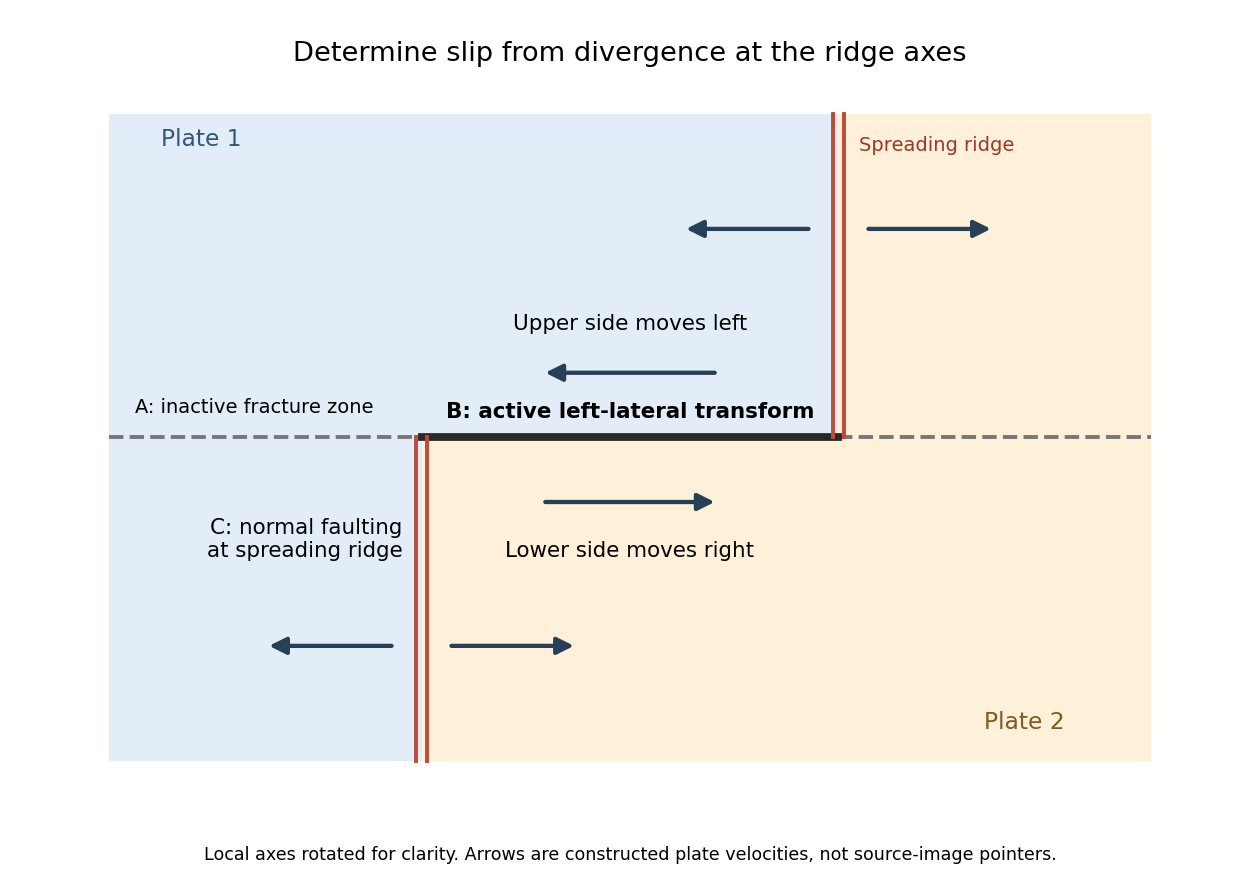
Why the active transform in the supplied geometry is left lateral
. Original idealized plan-view construction using the supplied ridge arrangement and relative motion directions. It illustrates the kinematic test, rather than reproducing the exam bathymetry. Details.
Probably yes in connected fractures or transiently opened pore space, especially where a transform fault admits circulating seawater; a uniform water-filled porous layer several kilometres thick is not guaranteed. Porosity and permeability of a porous medium generally decrease as cracks close or seal, while ongoing faulting can reopen pathways. Fluid can occur at high pressure and temperature, including a supercritical state; it need not resemble cold surface water.
Several complementary tests address presence and origin:
- Geological: recover fresh cores or dredged fault rocks. Hydrous alteration assemblages, veins, serpentinite replacing peridotite, and altered gabbro record water-rock interaction. Sealed fluid inclusions can preserve former fluids. These establish fluid access in the past; they do not by themselves demonstrate currently connected free pore fluid.
- Geochemical: analyse sampled fluids and fluid inclusions for salinity and chlorine, oxygen and hydrogen isotope ratios, and strontium or boron isotope ratios in alteration products. Compare with seawater, host rocks, and possible magmatic or metamorphic sources. A seawater-like input modified systematically by water-rock interaction supports deep circulation from the ocean. Exchange, isotope fractionation, mixing and phase separation mean that altered fluids need not retain the exact surface composition.
- Geophysical: combine seismic tomography, Compressional-to-shear wave speed ratio and seismic attenuation with magnetotelluric sounding or controlled-source electrical measurements. A connected saline fluid network can reduce electrical resistivity and change elastic wave speeds. Sample hydrothermal vents, measure heat flux and, if drilling is possible, make direct pore pressure and permeability measurements.
No one anomaly uniquely identifies water. Seismic velocity can also reflect cracks, composition and temperature; electrical conductivity can reflect melt or conductive minerals. Serpentinization demonstrates incorporation of water into minerals, which must be distinguished from fluid currently occupying pore space. At an oceanic transform fault, an external seawater supply is the natural first hypothesis, but isotope ratios and chemical budgets can test contributions from deep fluids rather than presuming the source. A research example of coupled deformation and hydrothermal alteration is Mass transfer and fluid flow during detachment faulting and development of an oceanic core complex, Atlantis Massif by Chiara Boschi and others; a detachment system illustrates the methods without proving identical flow at every transform fault.
Cooling makes the oceanic lithosphere denser and contracts it; isostatic adjustment therefore lowers the seafloor. The cooling layer includes substantial mantle, not just the approximately fixed-thickness igneous oceanic crust.
New plate near a spreading ridge is hot and relatively buoyant. As it moves away, conductive cooling penetrates more deeply, and material formerly in the hot asthenosphere becomes part of the colder thermal boundary layer. To first order,where is the volumetric thermal expansion coefficient, a reference mantle density, the hot reference temperature, and plate age. A positive depth-integrated density anomaly makes the column negatively buoyant relative to the ridge column. Isostasy is restored by downward displacement and mantle redistribution; cold rock also occupies less volume.
At a fixed sufficiently deep datum, deepening the seafloor by removes an equivalent thickness of rock from the column and replaces it with less dense seawater. In the usual constant-property approximation this giveswhere is seawater density and lies below the relevant thermal anomaly. This explains why contraction alone and water-loaded seafloor subsidence are not identical numerical quantities.
For a half-space cooling model,so integration yieldsHere is thermal diffusivity and is measured downward from the surface of the thermal model. The leading oceanic thermal subsidence is proportional to . A finite oceanic plate cooling model limits this growth at old ages. Sediment loading, dynamic topography, anomalous crust thickness and hydrothermal heat transport can produce departures from the simple relation.[ref]
Choose a common horizontal compensation depth beneath the deepest cooling-induced density anomaly, within mantle that can relax pressure differences over the timescale considered. In a normal oceanic plate model, this means below the old plate's thermal lithosphere, not at the base of the approximately 7 km thick oceanic crust.
The reason is that cooling changes density through both crust and lithospheric mantle. A datum at the Mohorovičić discontinuity would omit most of the changing column mass. A different datum for each age would also compare unlike columns. Once the common datum is sufficiently deep, extending it farther into laterally uniform mantle adds the same mass per unit area to each column and does not change the predicted relative subsidence.
There is no unique number fixed by the question. For an illustrative oceanic plate cooling model with a thermal thickness about 100–125 km, a common datum beneath that layer, of order 150–200 km below sea level, is a defensible choice provided the model has no substantial lateral density anomaly there. These are model choices, not measured universal boundaries. In a half-space cooling model, use the oldest age to choose a practical cutoff: makes the remaining temperature anomaly less than about 0.5% of its surface contrast. For and million years, this is about 225 km. A half-space model has no mathematically sharp finite thermal base.
Finally, equal column mass is the local, approximately constant-gravitational acceleration representation of equal pressure at the datum. A weak asthenosphere permits pressure relaxation through slow solid-state material creep; it need not be liquid. Short-wavelength loads, lithospheric flexure or dynamic topography can violate local column-by-column isostasy, requiring a more complete mechanical model.
I would not assign the lunar mare an automatic terrestrial 100–125 km compensation level. For present-day mare basins, a local equal-column-mass model may have no physically valid compensation depth; first test whether lithospheric flexure supports the load. For ancient thermally driven subsidence that did relax, choose a common datum beneath the cooling layer in deformable lunar mantle appropriate to that epoch.
The Moon is smaller than Earth and has lost a larger fraction of its original heat. Its cold, mechanically strong outer shell can be much thicker relative to its radius than the terrestrial oceanic lithosphere. Lunar mare basalts filled pre-existing impact basins: their loading, basin excavation, mantle uplift, cooling and the evolving strength of the lithosphere all matter. A thick elastic lithosphere can support lateral stress differences, so equal column mass need not hold even after a long time. The strong gravity anomalies of lunar mascons, measured by GRAIL, are evidence that the present mare-basin system is not everywhere locally compensated.[ref]
For an explicitly assumed ancient relaxed thermal model, estimate its thermal penetration depth from thermal diffusivity and the elapsed cooling time, infer the contemporaneous mechanical lid from gravity-topography admittance or basin deformation, and place below that layer where lateral pressure anomalies relax. For example, a hypothetical several-hundred-kilometre-thick lid requires a deeper datum than that lid, not the shallow crust-mantle boundary. The paper supplies neither an epoch-specific thermal model nor a load wavelength, so a unique kilometre value is not determined. If the chosen datum is a substantial fraction of the lunar radius, spherical geometry and radial variation in gravity must replace the flat, constant-gravity column approximation.
Does the Moon have an asthenosphere? Not a demonstrated shallow, globally connected Earth-like layer underlying mobile plates; but “no weak or partially molten mantle anywhere, ever” is too strong. Apollo lunar seismology indicates a cold outer interior and more attenuating deep regions. Reanalyses support a deep low-velocity or partially molten region near the lunar core, while lunar laser ranging and tidal Love numbers constrain deep deformability and tidal dissipation. Such a deep weak region is sometimes called a lunar asthenosphere; it is not automatically the correct local compensation surface for a mare load.[ref]
The inferred melt fraction and distribution remain model dependent: Dissipation at tidal and seismic frequencies in a melt-free Moon by Francis Nimmo and others demonstrates that much of the dissipation can also be explained by hot solid-state anelasticity, although its model does not reproduce every frequency-dependent constraint. The Moon was hotter during mare emplacement and could relax loads differently then. Choose the datum from the relevant thermal and mechanical history, or use a flexural model when local isostasy fails.
Articles by others on the same topic
There are currently no matching articles.