Take positive toward positive from the downward vertical, as in the source diagram. The mass has position and velocityThus and . Expanding the squared speed givesThe prescribed support coordinates are functions of time, rather than additional dynamical variables. Terms depending only on time do not affect the Euler-Lagrange equation for , but have been retained here to obtain the inertial-frame kinetic and potential energies directly.
The derivatives needed in the Euler-Lagrange equation areThe terms proportional to cancel after differentiation, leavingWith and ,Hence the vector equation is . In the translating support frame, is the inertial force. The rod's tension passes through the hinge and contributes no torque about it. The same torque equation therefore has an immediate mechanical interpretation.
For horizontal forcing the exact angular equation isWrite with slowly varying and . To leading order in the slow-to-fast frequency ratio, , which balances the rapid forcing. Expand the right-hand side to first order in :During one fast period treat as fixed. The averages and vanish, whereasThe leading averaged equation is thereforeThe effective force comes from correlation between the rapid displacement and the rapidly varying driving torque; simply averaging the driving cosine to zero misses it. This keeps the leading nonzero fast-motion contribution, proportional to , while neglecting terms suppressed by additional powers of or of the slow rate divided by . The gravitational expansion at order is smaller in the stated high-frequency regime. The resulting slow frequencies must also remain small compared with for averaging to be self-consistent.
For a fixed-pivot pendulum the angular inertia is , so . Integrating the averaged force gives, up to an arbitrary additive constant,Linearizing about givesHence the downward state becomes linearly unstable forAt its quadratic restoring term vanishes: the leading quartic coefficient is positive, so it is marginal at linear order, rather than already a local maximum. Above threshold the two stable tilted equilibria satisfy . Horizontal vibration therefore destabilizes the downward orientation and produces tilted minima; it does not stabilize the upward orientation in this model. Because , the threshold is compatible with the assumed small support excursion.
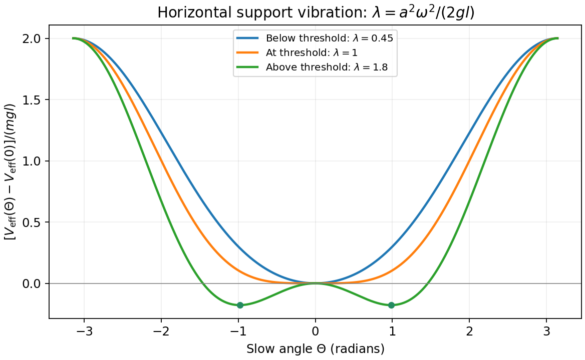
Original averaged pendulum potentials below, at and above the horizontal-vibration instability threshold
. Details. Every element of the uniformly distributed mass has speed squared , so the total kinetic energy is . The extension of the ring's full circumference is , and the stated spring constant therefore givesThe magnetic coupling for each charge element is . With the symmetric gauge and tangential speed , integration over the ring gives . ThusThis idealization neglects charge self-energy, radiation and deformation away from a circular ring. The elastic constant refers to extension of the whole circumference; replacing it by a radial spring constant without the factor changes the problem.
The canonical momenta areThe Legendre transform cancels the velocity-linear magnetic term, giving the energy expressed in velocities,But Hamilton's equations differentiate with respect to canonical coordinates and momenta, not velocities. In its proper canonical variables the same Hamiltonian isIt explicitly contains because canonical angular momentum differs from mechanical angular momentum. This reconciles magnetic forces with the absence of magnetic work: the magnetic field can exchange radial and tangential motion without changing the total mechanical energy.
Time-translation symmetry conserves the energy , and axial rotational symmetry makes a cyclic coordinate, conservingThe radial Euler-Lagrange equation before elimination isInsert . The cross terms linear in cancel, leavingEquivalently use the reduced radial potentialThe last term is constant at fixed and has no radial derivative, but is part of the full conserved energy. Conservation of is stated in the rotationally symmetric gauge; the conserved mechanical combination can be written in terms of magnetic flux in a gauge-independent way.
The initial angular velocity cancels the flux term in the canonical angular momentum:Define and . The radial equation becomes , soThese identify the paper's with . For nonzero radius, also fixesA radius is nonnegative. The formal sinusoidal solution remains strictly positive for a full cycle only if , or . At equality it touches zero; at stronger magnetic coupling it first reaches zero and its negative continuation is not a physical ring radius. No collision or re-expansion rule at collapse is supplied, so the circular-ring solution is then valid only up to the first zero. This domain qualification leaves the requested differential-equation solution intact.
Take the stated negligible-natural-radius limit as , with both initial velocities zero at . Then . Write and , where . At two radial turning points , equality of the effective radial energies givesUsing gives, for and ,The minimum is a regular radial turning point, soThe angular velocity has the sign of . On the initial inward motion, conservation of canonical angular momentum produces the rotation needed to prevent collapse to zero radius.
The strictly zero-field case is singular for this angular formula: and the ring instead collapses to with inward radial speed in the ideal radial equation, where an angular coordinate ceases to describe a ring. The limit through nonzero fields gives a tiny positive turning radius with large angular velocity, and must not be substituted into the formula at exactly zero field. A small nonzero also matters if the predicted minimum becomes comparable with it.
For canonical coordinates , the Poisson bracket isIt is bilinear and antisymmetric, obeys the Leibniz rule in either argument, and satisfies the Jacobi identity. These properties encode the symplectic structure of phase space. The two printed inline applications are treated separately below.
An invertible change is canonical when it preserves the Poisson bracket. Its fundamental brackets must beThe chain rule then makes the bracket of any two observables identical in the old and new coordinates. Consequently Hamilton's equations retain their canonical form. A time-dependent canonical transformation also requires the corresponding extra term in the transformed Hamiltonian; bracket preservation by itself concerns each fixed time.
Along Hamiltonian motion,Substituting and givesFor the printed there is no explicit time term. In particular, an autonomous observable is conserved when its Poisson bracket with vanishes. Taking or recovers Hamilton's equations.
For ,The derivatives of are and . Its Poisson bracket with is thereforeDirect differentiation, , gives the same expression and checks the bracket sign.
In one canonical degree of freedom it is enough to check for a locally invertible transformation. Hereso and . To obtain exactly the requested Hamiltonian, choose and the positive branch for :The identities and giveThis is a local canonical chart, with inverseIt is not a global identification of the real half-plane with the entire oscillator plane. The negative branch for gives the analogous lower wedge. This domain matters if an oscillator trajectory is continued beyond the boundary of the chart.
The perturbed Hamiltonian is . Hamilton's equations give , , henceIn the paper's time units the natural frequency is one. The retarded Green function is : it vanishes before the source, is continuous at zero and has a unit derivative jump there. With Fourier convention ,Both real-frequency poles are displaced below the real axis. Causality therefore selects the convolutionFor the exponential rises as throughout the integral. For , split the integral at . Evaluation yieldsThe response is nonzero before because the prescribed force is already nonzero then; this does not violate causality. Both and are continuous at zero. The force eventually decays, leaving the free oscillation . A general solution adds , but the retarded condition of no incoming free oscillation as fixes .
The oscillator equation is well-defined on the full plane. Interpreted through the positive- chart of part (c), it describes the original real variables only while , with . The requested retarded oscillator solution is a continuation in the new variables; it is not a claim that this canonical chart remains valid at all times for every .
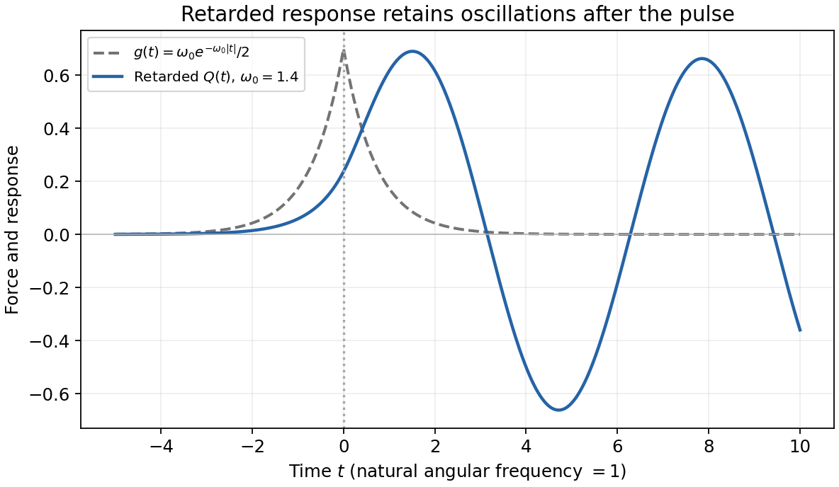
Original retarded response to a two-sided exponential force; the pre-zero response follows earlier nonzero forcing
. Details. An element with unperturbed coordinate length has mass and transverse speed squared . Its actual length isAt fixed tension the extra elastic energy to this order is . Subtracting it from the kinetic energy givesHere prime means and dot means . The approximation retains quadratic transverse energy and neglects higher-order slope effects and longitudinal motion. The resulting field equations are for , with wave speed when .
Adding a constant to changes neither its time nor space derivatives, so the action is invariant. The associated Noether density and flux areThe wave equation gives . ThereforeThis is total physical transverse momentum. It is conserved for a whole isolated infinite string with vanishing boundary flux, periodic boundary conditions, or endpoints exerting no net transverse force. For a finite subsystem momentum can flow through its ends, and fixed supports can exchange momentum with the string. Thus the local conservation law always holds in this model, while constancy of the integrated charge requires the stated boundary condition.
An infinitesimal rotation about gives and . Both the squared transverse velocity and squared transverse slope are rotational invariants. Noether's theorem therefore givesDifferentiating and using the two wave equations givesConsequently is the angular momentum about the equilibrium string axis, conserved when the net endpoint torque flux vanishes. For a finite segment, . It is not momentum associated with translating the coordinate ; its symmetry rotates the two physical transverse displacement components into one another.
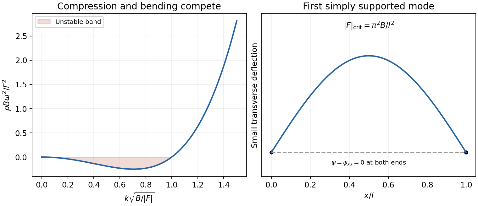
For one transverse displacement the density isIts variation is . Integrating once in time and twice in space gives the bulk coefficientThe spatial boundary contribution is integrated over time. ThusInsert to obtainFor compression , sufficiently long waves have and grow exponentially. Positive bending rigidity stabilizes short wavelengths; without it the compressed small-slope model would have no short-wavelength regularization.
With endpoints held at zero displacement but free to rotate, variation permits arbitrary endpoint and gives the natural zero-moment condition there. These are simply supported endpoints. The normal modes areThe first mode becomes unstable when , soEquivalently the compressive load exceeds . At equality the linear mode is neutral and nonlinear terms are needed to determine its post-buckling amplitude. The quadratic energy of is , giving the same sign test.
The endpoint displacement condition alone does not impose clamping. The quoted threshold uses the natural free-slope boundary condition of the stated variational problem. If rotations were also fixed, the admissible modes and threshold would change; one must not import a clamped-end formula into this result.


Use , signature , and define . Under a local phase transformation,the derivative of the phase cancels the change of the potential, giving . Therefore a gauge-invariant scalar-electromagnetic Lagrangian density isThe mass term is invariant, the covariant-derivative product has canceling phases, and because mixed partial derivatives commute. A potential depending only on may be added without changing the symmetry. The Maxwell term makes the electromagnetic field dynamical; it can be omitted when is a prescribed external background.
Expanding the covariant-derivative term gives the interaction linear in plus . This quadratic term is required for exact local gauge invariance. The later part (c) deliberately gives only the linear interaction, and must be solved as that different stated Lagrangian rather than silently adding the missing term.
For fields and a continuous infinitesimal internal symmetry , suppose the density changes by a divergence, . Varying the action and using the Euler-Lagrange equations gives the Noether currentThe conserved charge is when the flux through the boundary vanishes; more generally . If the Lagrangian is exactly invariant, . Treat a complex field and its conjugate as independent variables during variation, imposing conjugacy on physical solutions. Time and space translations give energy and momentum through the corresponding spacetime version of the theorem. Continuous global symmetry gives an ordinary charge; local gauge redundancy requires additional care and is not an independent conserved charge for every arbitrary function.
Treat and as independent fields, keep as the prescribed background, and use the source's interaction with no added term. The momentum derivatives areVarying and gives respectivelyNo Lorenz gauge condition has been assumed. The background divergence term must be retained unless such a condition is separately imposed.
The canonical momenta conjugate to the two scalar fields areso and . Define the physical three-vector potential by . The Legendre transform in the proper canonical variables isEquivalently the first product is . The last quadratic term arises from replacing velocities by canonical momenta even though the original Lagrangian has no quadratic interaction. It is not permission to modify the specified Lagrangian. An explicitly time-dependent background generally makes the scalar-field energy time dependent.
For and , the interaction is invariant under the constant phase because every product has net zero phase. Applying the Noether formula to the two independent fields givesThe sign corresponds to the printed transformation . Reversing the phase parameter would reverse the entire current, with no change in conservation.
The derivative products in the divergence of the first term cancel pairwise:The two field equations from part (c) implyMultiplication by exactly cancels the remaining background terms, proving without requiring to be constant or divergence free. The global phase symmetry survives even though this truncated interaction is not exactly invariant under arbitrary local gauge transformations.
Mean-field theory replaces fluctuating interactions with the average field produced by the other degrees of freedom. For an interacting spin system, write and neglect connected products . This reduces the many-body partition function to independent single-site factors coupled through a self-consistency equation for .
The approximation is most reliable when many effectively independent neighbors contribute, for sufficiently long-range interactions, or above the upper critical dimension away from the fluctuation-dominated critical region. It usually becomes least reliable near a continuous transition in low dimensions, where correlations extend over long distances. It can estimate ordering scales and reveal candidate broken symmetries while giving incorrect critical exponents or even a spurious transition. The two-dimensional isotropic model in the later parts is an especially important example of this limitation.
Let the coordination number be , and choose the spin-space axis along . The mean-field decoupling of a bond isThe original directed neighbor sum counts each bond twice, so its factor cancels that double counting. The resulting energy isThe constant prevents double counting of the mean interaction energy and is necessary if free energy is minimized with respect to . With the source's unnormalized solid-angle measure, the single-site integral isThereforeAt take . A normalized solid-angle measure would remove the factor without changing the self-consistency equation. These are three-component classical spins on a two-dimensional positional lattice, not spins constrained to a plane.
The PDF's hint is a correct angular-integration identity for a term with coefficient . That coefficient is not the full single-site molecular field after summing all four neighbors and decoupling both entries of each bond. The net coefficient is , as follows from the explicitly stated Hamiltonian; inserting the hint's coefficient as the total field would lose the coordination and double-counting factors.
In mean-field theory all sites have the same normalized single-site distribution . Consequentlywhere is the Langevin function. Requiring the average used to construct the field to equal the average in that field givesSetSince , the self-consistency equation is exactly . It also follows by stationarity of . This independent route checks the constant term and all neighbor-counting factors in the partition function.
Near zero the Langevin function has expansionFor positive , rises toward one and its ratio decreases from to zero. Therefore a line has only the zero intersection for , and also a nonzero positive intersection for . In a fixed signed component there is a corresponding negative solution; in the isotropic vector problem the nonzero solutions have all spin-space orientations.
The mean-field transition temperature isAt the critical temperature the line is tangent at the origin. Just below it, , the usual mean-field square-root onset. The ordered minimum is stable below this temperature while becomes unstable.
This is a mean-field prediction, not a genuine finite-temperature ordering transition for the ideal two-dimensional short-range isotropic model. Long-wavelength spin fluctuations invalidate the predicted nonzero thermodynamic magnetization at every . The relevant obstruction is the Mermin-Wagner theorem for continuous spin symmetry; anisotropy, long-range interactions or a finite sample change the assumptions. Its original paper establishes the absence of finite-temperature magnetic ordering for one- and two-dimensional finite-range isotropic Heisenberg models.[ref]
Absence of Ferromagnetism or Antiferromagnetism in One- or Two-Dimensional Isotropic Heisenberg Models by N. D. Mermin and H. Wagner. Physical Review Letters 17, 1133 (1966), abstract; physical limitation of finite-temperature mean-field order
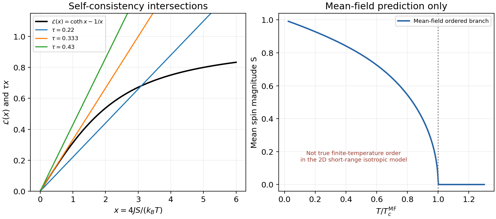
Original Langevin self-consistency plot and the mean-field order parameter, explicitly distinguished from true two-dimensional isotropic long-range order
. Details. 
For uniform unconstrained boundary conditions, the positive gradient coefficient favors a spatially constant minimizer. Put . The remaining free-energy difference is . Its minimum isBelow the amplitude is fixed but its direction is arbitrary; the set of uniform minima is a two-sphere. The free-energy minimum is below and above. The order parameter vanishes continuously, so this is a continuous, second-order transition within Landau theory.
The free energy has internal spin-rotation/reflection symmetry; a chosen nonzero vector leaves an subgroup invariant. Restricting to proper rotations, this is spontaneous symmetry breaking. There are two transverse orientation directions and a massive amplitude direction below the transition. Spatially varying directions cost gradient energy, and imposed boundaries or defects can prevent a uniform minimizer. In strictly two-dimensional equilibrium with short-range interactions, the fluctuation caveat of part (d) still applies: minimizing this polynomial functional at mean-field level does not overturn the absence of finite-temperature spontaneous magnetization.
Articles by others on the same topic
There are currently no matching articles.