Past exam of the theoretical physics I course of the University of Cambridge / 2018

Choose Minkowski metric $(+,-,-,-)$, so $A_{\mu }=(\varphi /c,-\mathbf{A})$ and $d\tau =dt\sqrt{1-v^2/c^2}$. In laboratory time the relativistic charged-particle action has LagrangianHere $e$ denotes the signed particle charge in the action. The canonical momentum and the position derivative areThe Euler-Lagrange equation therefore givesThe last term is $(\mathbf{v}\times \mathbf{B}{)}_i$, and the first two terms form the electric field. Thus the relativistic Lorentz force equation isIts power relation and acceleration form areThe power relation follows by taking the scalar product with $\mathbf{v}$ and using the relativistic energy-momentum relation. It also shows why the magnetic field alone cannot change the particle's energy.

For a uniform constant electric field and zero magnetic field, the mechanical momentum changes linearly even though the velocity does not:Invert $\mathbf{p}=m\gamma \mathbf{v}$ using $\gamma =\sqrt{1+p^2/(m^2{c}^2)}$. The result for arbitrary initial direction isEquivalently, $\mathbf{v}=c\mathbf{p}/\sqrt{m^2{c}^2+p^2}$. This gives $\mathbf{v}(0)={\mathbf{v}}_0$ and guarantees $|\mathbf{v}|<c$ at every finite momentum. The transverse momentum stays constant, but its velocity component generally decreases because the Lorentz factor increases. Thus an initial transverse velocity must not be treated as constant during the electric acceleration; this is the relativistic motion in a constant electric field with transverse momentum effect.

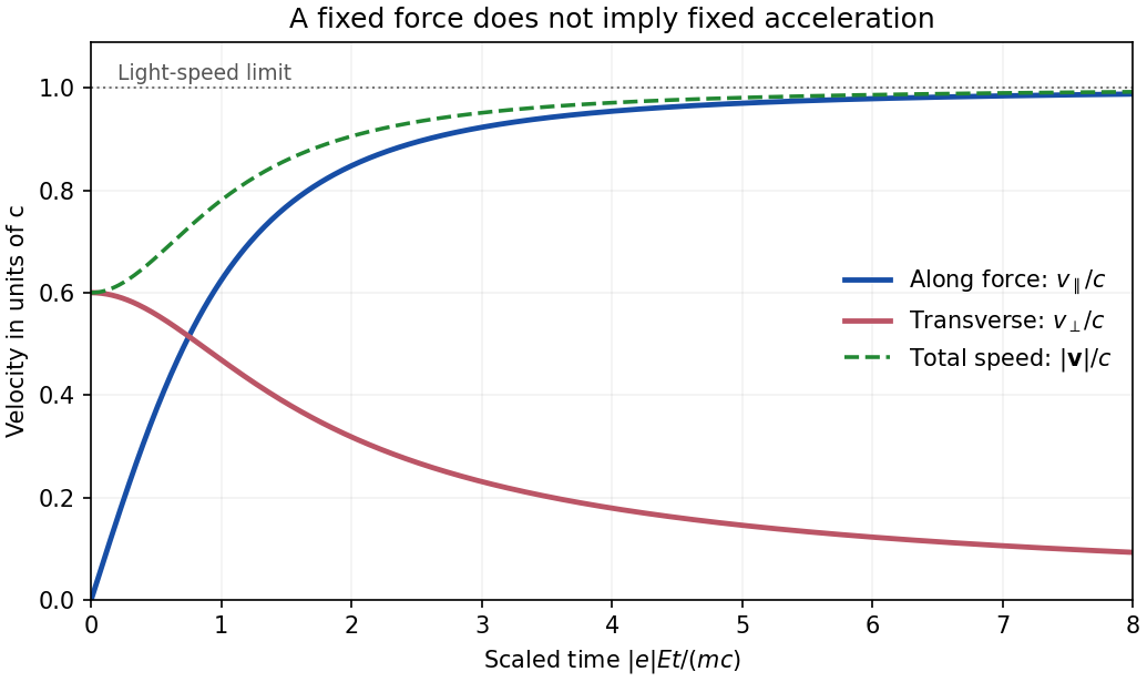
If $e\mathbf{E}\ne 0$, then $\mathbf{p}(t)=e\mathbf{E}t+O(1)$, and the relativistic energy-momentum relation givesThe particle approaches the speed of light in the direction of the electric force, independently of its initial velocity. For positive $e$ the limiting direction is along $\mathbf{E}$; for negative $e$ it is opposite. A massive particle never reaches that limiting speed in finite time. If the force is zero, the velocity remains ${\mathbf{v}}_0$ instead.

With no electric field, the power relation from part (a) givesConsequentlyThe magnetic part of the relativistic Lorentz force changes the direction of mechanical momentum, but performs no work. This conclusion does not require the magnetic field to be spatially uniform: it follows from the local orthogonality of $\mathbf{v}$ and $\mathbf{v}\times \mathbf{B}$.

Let $\mathbf{b}=\mathbf{B}/B$ for a nonzero constant magnetic field. Since $\gamma$ is constant, the relativistic Lorentz force reduces toThe projection along $\mathbf{b}$ is constant. In the perpendicular plane define the signed cyclotron frequency $\Omega =eB/(m{\gamma }_0)$; thenThe explicit rotating velocity isThis is the relativistic cyclotron orbit frequency in laboratory time, reduced from the nonrelativistic frequency by $1/{\gamma }_0$. With nonzero parallel velocity, the trajectory is a helix. If ${\mathbf{v}}_{\perp 0}=0$, that perpendicular vector stays zero and has no nontrivial fundamental period; the displayed $T$ is the period of a nonzero transverse orbit.

Use the downward $y$ direction of the PDF diagram. The bob's Cartesian coordinates areThusThe hinge and rod are massless, so only the bob contributes kinetic energy:Because gravity points along positive $y$, its gravitational potential energy is $-mgy=-mg\ell \cos \theta$. The zero-rest-length spring has elastic potential energy $k{s}^2/2$. Put $s=\ell \eta$ and divide $T-V$ by the positive constant $m{\ell }^2$. The equivalent Lagrangian isMultiplying the action by a nonzero constant leaves its stationary paths unchanged. This derivation is a direct use of kinetic energy from Cartesian position vectors; no independent kinetic term should be assigned to the massless support.

For the horizontal generalized coordinate $\eta$,The corresponding Euler-Lagrange equation isFor $\theta$, the terms proportional to $\dot{\eta }\dot{\theta }\sin \theta$ cancel between $d(\partial L/\partial \dot{\theta })/dt$ and $\partial L/\partial \theta$. Hence the other exact equation isKeeping only terms linear in small coordinates and their derivatives givesThe equilibrium is $\theta =\eta =0$. These characteristic frequencies label gravitational and spring restoring scales; they are not two independent normal mode frequencies of this massless-support system.

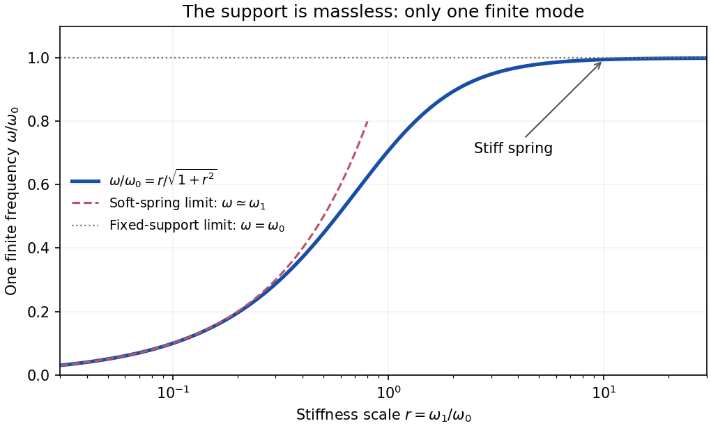
Subtracting the two linearized equations eliminates their acceleration terms:For $g,k>0$, the assumed nontrivial simple harmonic motion therefore hasThe support displacement and pendulum angle oscillate in phase. Inserting this relation into either Euler-Lagrange equation yieldsso the one positive finite angular frequency isThe negative frequency describes the same real oscillation after a phase change. For a general phase, replace the sine in both coordinates by $A\cos (\omega t)+B\sin (\omega t)$.

There is no missing second finite branch. The quadratic Lagrangian iswhose kinetic matrix is $\left(\begin{array}{cc}1& 1\\ 1& 1\end{array}\right)$ and has rank one. Its characteristic determinant is ${\omega }_0^2{\omega }_1^2-({\omega }_0^2+{\omega }_1^2){\omega }^2$, not a quadratic polynomial in ${\omega }^2$. This singular kinetic matrix in small oscillations results from taking the support mass to be exactly zero. Adding a small support mass restores a second mode that runs to infinite frequency as that mass vanishes.

For a stiff spring,The hinge becomes fixed, recovering the simple pendulum frequency, as expected for the pendulum with a massless spring-mounted support. At finite $k$, horizontal support motion makes the frequency smaller.

If $L^{\prime }=L+dF(q,t)/dt$, the action changes by an endpoint term:In the principle of stationary action with fixed endpoints, $\delta q(t_i)=\delta q(t_f)=0$ and the endpoint times are fixed. Therefore $\delta (S^{\prime }-S)=0$, and the two actions give the same bulk Euler-Lagrange equations.

For a Lagrangian density, adding ${\partial }_{\mu }{K}^{\mu }$ changes the action by ${\int }_{\partial \Omega }{K}^{\mu }{n}_{\mu }d\Sigma$, by the divergence theorem. Its variation vanishes for compactly supported field variations, or when the appropriate boundary data are held fixed. These total divergences in a variational principle can therefore be discarded when deriving bulk equations under those conditions.

The qualification about boundaries matters: if $K^{\mu }$ depends on field derivatives, their variations on the boundary must also be controlled. A total derivative can change the canonical momenta or the chosen representative of a Noether current, even while leaving the bulk dynamics unchanged.

Let $P^{\mu }=\partial \mathcal{L}/\partial ({\partial }_{\mu }h)$ and $Q^{\mu \nu }=\partial \mathcal{L}/\partial ({\partial }_{\mu }{\partial }_{\nu }h)$. Define the second coefficient with ordered repeated indices and $Q^{\mu \nu }=Q^{\nu \mu }$, so thatThis convention avoids double-counting a mixed derivative such as $h_{,12}=h_{,21}$. The first derivative term needs one integration by parts. The second derivative term needs two:Combining the terms givesFor compactly supported variations, or fixed $\delta h$ and its first derivatives at the boundary, the last integral vanishes. The fundamental lemma of the calculus of variations then yields the Euler-Lagrange field equation with second derivatives:The plus sign of the final term comes from the two integrations by parts. In general this gives fourth-order equations, although the order in a particular coordinate depends on which second derivatives occur in the density.

Put $R=h_t-\nu {\nabla }^{2}h$, where the diffusion coefficient $\nu$ is constant. ThenOne temporal and two spatial integrations by parts givewith compactly supported variations. HenceHere ${\nabla }^4=({\nabla }^2{)}^2$ is the biharmonic operator. The cross terms cancel because $\nu$ is constant and spatial and temporal derivatives commute. Equivalently, $P^0=2R$ and $Q^{ij}=-2\nu R{\delta }^{ij}$ in part (b), producing $-2{\partial }_{t}R-2\nu {\nabla }^{2}R=0$.

This squared diffusion-residual action does not have only the first-order diffusion equation as its stationary equation. The zero-residual paths $h_t=\nu {\nabla }^{2}h$ have $S=0$ and are certainly solutions, but the variational equation is the higher-order one above. For a spatial Fourier mode with nonzero wavevector $\mathbf{k}$, it givesBoundary data or an additional physical selection principle are needed to retain only the decaying diffusion branch. The spatially uniform mode instead has $h_0(t)=A_0+B_{0}t$ in the stationary equation.

With constant $\nu$, the bulk action is invariant under time translations, translations in the two spatial coordinates, and rotations or reflections within the substrate plane. The Laplacian has no preferred direction, giving the planar $O(2)$ symmetry. It also has scalar-field shift symmetry $h\mapsto h+a$, expressing the arbitrary origin of height, and the discrete symmetry $h\mapsto -h$ because its residual is squared.

There is an additional exact tilt symmetry $h\mapsto h+\mathbf{b}\cdot \mathbf{x}$: the added slope is time independent and has zero Laplacian. More generally, adding any function $f$ satisfying $f_t=\nu {\nabla }^{2}f$ leaves the residual unchanged. Such bulk transformations need not preserve prescribed boundary conditions or a restricted physical interpretation of the height.

In two spatial dimensions the action also has the anisotropic scale invarianceThe spacetime measure scales as $b^4$ and the squared residual as $b^{-4}$. The time and length scales are therefore related diffusively, rather than by a Lorentz transformation.

Ordinary time reversal needs a boundary qualification. The identityshows that the density is time-reversal invariant up to a total divergence. Thus the bulk stationary equation $h_{tt}-{\nu }^2{\nabla }^{4}h=0$ is invariant under $t\mapsto -t$, although the printed density is not pointwise unchanged. The time reversal of the squared diffusion-residual action exchanges the growing and decaying branches; the selected first-order diffusion equation alone is not time-reversal invariant at fixed positive $\nu$.

The derivatives of the Lagrangian density are ${\mathcal{L}}_{\varphi }=0$, ${\mathcal{L}}_{{\varphi }_t}={\varphi }_t$, and ${\mathcal{L}}_{{\varphi }_x}=-{\varphi }_x$. The Euler-Lagrange field equation is thereforeThis is the one-dimensional wave equation with wave speed $c_s=\sqrt{\kappa /\rho }=1$. Both signs of propagation are allowed: $\varphi (x,t)=F(x-t)+H(x+t)$ for sufficiently regular profiles.

Use $x^{\mu }=(t,x)$ and Minkowski metric ${\eta }^{\mu \nu }=\mathrm{diag}(1,-1)$, with the wave speed equal to one. Regarding $\varphi$ as a scalar field, the symmetric canonical stress-energy tensor isIt obeys ${\partial }_{\mu }{T}^{\mu \nu }=0$ on the wave equation. For a scalar field the intrinsic spin current vanishes. The total orbital Lorentz current and its integrated angular-momentum tensor areBecause there is only one spatial dimension, its only independent possibly nonzero component iswhere $P=\int pdx$. The corresponding flux is ${\mathcal{J}}^{101}=t\mathcal{E}-xp$. Symmetry and conservation of $T$ giveThus $J^{01}$ is conserved provided the boundary flux vanishes and the integrals exist. For example, localized wave packets on an infinite line have this property. One can also check directly that $d\int x\mathcal{E}dx/dt=P$, so the two terms in $J^{01}$ have cancelling derivatives.

The significance is the boost charge of a one-dimensional scalar field. There is no independent spatial rotation or ordinary spatial angular-momentum component in one dimension. Instead, the action has the mathematical Lorentz invariance of a massless wave field with invariant speed $c_s=1$, and $J^{01}$ generates its boost. Its conservation says that the center of energy moves uniformly. This is a symmetry of the ideal wave-field model, rather than an assertion of fundamental vacuum Lorentz symmetry for a material rod. Fixed boundaries can break it, and a general solution with nonvanishing boundary flux need not conserve the integrated charge.

With the PDF's inverse Fourier transform convention, the derivatives act asso its forced differential operator becomes ${\omega }^2-k^2+i\gamma \omega k^2$. ThusFor the physical impulse response choose the retarded fundamental solution, vanishing before $t=0$. For $k\ne 0$ and $\gamma >0$, its poles lie in the lower half-plane. The retarded Fourier pole prescription $\omega \mapsto \omega +i0$ specifies the zero mode and the zero-damping limit as well; a Green function without a temporal or boundary prescription would otherwise permit homogeneous additions.

This is the Kelvin-Voigt rod Green function. Multiplying the homogeneous real-space equation by $-1$ givesA spatial Fourier mode therefore satisfies ${\ddot{\varphi }}_k+\gamma k^2{\dot{\varphi }}_k+k^2{\varphi }_k=0$: positive $\gamma$ really damps the motion. For sufficiently decaying fields its energy satisfiesThis checks the sign of the imaginary term in $\hat{G}$ independently of the transform calculation.

For $0<k^2<4/{\gamma }^2$, defineThe simple poles are ${\omega }_{\pm }=\pm {\Omega }_k-i{a}_k$. In the inverse transform $\tilde{G}(k,t)=\int e^{-i\omega t}\hat{G}d\omega /(2\pi )$, close the contour below for $t>0$. Its clockwise orientation gives $-i$ times the sum of residues. That sum isFor $t<0$, close above; there are no poles. The residue theorem therefore givesHere $\Theta$ is the Heaviside step function. At $k=0$ the continuous retarded limit is $-t\Theta (t)$. At critical damping, ${\Omega }_k\to 0$ likewise replaces $\sin ({\Omega }_{k}t)/{\Omega }_k$ by $t$; beyond the stated oscillatory range an imaginary ${\Omega }_k$ converts it to a hyperbolic sine. These continuations retain decaying temporal exponents.

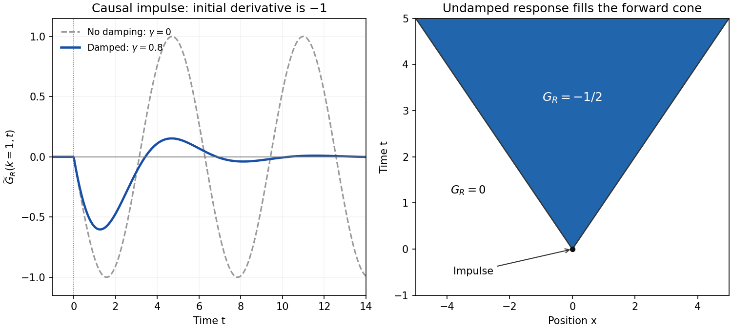
For each fixed $k$, taking $\gamma \to 0^{+}$ givesFor $t>0$, invert in space and set $s=kt$:The correctly normalized sinc function transform isFor instance, $\sin s/s=\frac{1}{2}{\int }_{-1}^1{e}^{isy}dy$, and Fourier inversion immediately gives the factor $\pi$. The PDF's prefactor $\sqrt{2/\pi }$ is inconsistent with its top hat of unit height; it would give height $\sqrt{2\pi }$. Using the normalized identity yieldsas a distribution. The values assigned precisely at a wave front do not change that distribution. This is the negative of the standard one-dimensional retarded wave Green function, because the PDF's differential operator is $-{\partial }_t^2+{\partial }_x^2$.

The sign and initial data can be checked without any contour calculation. Integrating the spatial-Fourier equation through the impulse givesIn real space these are $G_R(x,0^{+})=0$ and ${\partial }_t{G}_R(x,0^{+})=-\delta (x)$. In particular,for a smooth test function $f$, confirming the negative delta-function initial velocity. Before the impulse the displacement and velocity are zero. The disturbance fills the forward causal cone for the constant-speed wave equation, whose fronts move at unit speed, consistent with $\rho =\kappa =1$. The final question's printed $\rho =k$ is interpreted as $\rho =\kappa$, referring to the elastic constant, not to the Fourier wavevector. No initial conditions were otherwise specified, so the causal choice has been made explicitly.