Original examination: Functional programming, data structures and algorithms, procedural programming, and digital hardware examination paper by the University of Oxford (2005).
The map function transforms each head and recursively processes the tail. A right fold combines a head with the result for its tail, whereas a left fold passes an updated accumulator into the recursive call. In Haskell:
import Prelude hiding (map, foldr, foldl, concat)

map f [] = []
map f (x:xs) = f x : map f xs

foldr op e [] = e
foldr op e (x:xs) = op x (foldr op e xs)

foldl op e [] = e
foldl op e (x:xs) = foldl op (op e x) xs

concat = foldr (++) []
The last right fold uses list concatenation to replace each outer cons by appending its inner list. Thus
concat [xs,ys,zs] = xs ++ (ys ++ (zs ++ [])). Its right fold association matters: appending a list traverses its left spine, so these equations traverse each inner spine once on finite inputs. The concise answer isLet mean
concat (map f zss) = f (concat zss). We use structural induction on lazy lists, including the bottom value and allowing arbitrary, possibly partial, inner lists.For
[], the left side is [] and the right side is f [] = []. For the bottom value , both map f and concat are strict functions in the outer spine, and the supplied strictness of makes the right side too.For the cons case, assume and write the new head as
xs. The defining equations and the induction hypothesis giveThe third equality is exactly the supplied list concatenation preservation law. No inspection of xs was required, so the argument includes partial inner lists and undefined elements.This proves the identity for every finite outer spine ending in either
[] or . In the usual pure Haskell semantics, these functions are Scott continuous maps. An infinite outer list is obtained as a limit by finite approximation of a lazy list; both composite functions preserve that limit. Equality on all its finite approximations therefore gives equality on the infinite outer list. Equivalently, is an admissible predicate on lazy lists. ConsequentlyThe continuity assumption is the usual semantic assumption for definable functions here; an extension from finite to infinite inputs cannot be justified by ordinary finite induction alone.Use function extensionality: show for every value of the argument type. In lazy evaluation semantics, “every value” includes the bottom value and partial values. For list arguments, structural induction on lazy lists supplies the empty, bottom and cons cases, with continuity justifying passage to infinite lists.
The original printed equation has the same right fold on both sides, including the same operator and seed; this is visible in the scan.[ref]
Functional programming, data structures and algorithms, procedural programming, and digital hardware examination paper by the University of Oxford (2005). Printed p. 2, Question 1(c), displayed equation
Thus its literal answer isFor every input , both sides denote the very same expression foldr (oplus) e xs; equality follows by reflexivity. This remains true if its value is . Neither termination nor associativity nor an identity law is required. The scan does not establish a different intended equation, so no replacement by a left fold is assumed.Let be the two input lengths and suppose numeric comparisons cost constant time. The list-based set representation determines which representation invariant each answer must preserve.
For unsorted lists allowing repetition, retain every left-hand occurrence whose value appears on the right for set intersection, and use list concatenation for set union:
interR xs ys = [x | x <- xs, x `elem` ys]
unionR xs ys = xs ++ ys
The resulting lists represent exactly the desired sets; repeated entries are permitted. Membership by sequential search makes
interR take time complexity in the worst case. The list concatenation in unionR costs to build its copied left spine and shares ys; fully enumerating the resulting list costs .For unsorted, duplicate-free inputs, the same intersection keeps uniqueness, while the union retains
xs and appends only right-hand elements absent from xs:interU xs ys = [x | x <- xs, x `elem` ys]
unionU xs ys = xs ++ [y | y <- ys, not (y `elem` xs)]Neither filtered list has internal repetitions, and the filter in
unionU also excludes overlap with xs. Both operations have worst-case time complexity, customarily written when both lengths are positive. Using the original xs for each membership test avoids searching an ever-growing output.interS [] ys = []
interS xs [] = []
interS (x:xs) (y:ys)
| x < y = interS xs (y:ys)
| x > y = interS (x:xs) ys
| otherwise = x : interS xs ys
unionS [] ys = ys
unionS xs [] = xs
unionS (x:xs) (y:ys)
| x < y = x : unionS xs (y:ys)
| x > y = y : unionS (x:xs) ys
| otherwise = x : unionS xs ysWhen , sortedness proves that cannot occur anywhere in the right list, so it can be discarded from the set intersection or immediately emitted to the set union. The symmetric argument handles ; equal heads are consumed together. Each step consumes at least one input head, so both have worst-case time complexity. These bounds assume the sorted representation invariant is already established; sorting arbitrary inputs has its own cost.
| Representation | Set intersection | Set union, including output traversal |
|---|---|---|
| Unsorted, repetitions allowed | ||
| Unsorted, unique | ||
| Sorted, unique |
Use permutation generation by insertion: recursively arrange the tail, then insert the removed head in every possible position.
inserts x [] = [[x]]
inserts x (y:ys) = (x:y:ys) : map (y:) (inserts x ys)

perms [] = [[]]
perms (x:xs) = concat (map (inserts x) (perms xs))
The map function in
inserts prefixes y to each placement after the first position. For a list of length , the number of results obeys and , so mathematical induction gives . Every result still contains the same old elements and the one inserted element.Let be the length of
perms xs for an input of length . There is exactly one permutation of the empty list, namely the empty list itself: hence perms [] is [[]], with length one. For a nonempty input, each recursively obtained permutation has length and gives placements. ThusLength alone would not exclude repeated answers. Since the input elements are distinct, removing the distinguished element from any result uniquely recovers both its placement and the shorter permutation. Hence different construction choices give different outputs, and every desired permutation is obtained by inserting into its restriction to xs. For [a,b,c], this code yields [a,b,c], [b,a,c], [b,c,a], [a,c,b], [c,a,b], [c,b,a], each exactly once.To agree with the example, preserve the first occurrence of each value. This first-occurrence duplicate removal is a right fold:
remalldups = foldr step []
  where step x ys = x : filter (/= x) ys
The folded tail has no repetitions by the induction hypothesis. The list filter removes any occurrence of the new head from that tail; prepending the head then gives exactly one occurrence of it, in its first input position. Other values retain their relative order. For the supplied example the intermediate folded results, from right to left, are
[1], [3,1], [2,3,1], and [1,2,3]. ThusUnder lazy evaluation, constructing x : ... does not first demand the folded tail. That observation is essential for the infinite cases below. The alternative step that first asks whether x belongs to the folded tail would lose this property and would also keep last occurrences instead of matching the stated example.Assume a proper lazy list with defined elements and terminating equality tests. If infinitely many distinct values occur, first-occurrence duplicate removal produces an infinite list of distinct values, in first-occurrence order. To produce the next new value after have appeared, the nested list filters need skip only a finite input prefix: an infinite collection of distinct values cannot all belong to the already seen. The next new value therefore occurs at a finite position and is reached in finite work. ConsequentlyThis is a stream productivity claim, not a bounded-delay claim: arbitrarily long runs of repetitions can make successive delays arbitrarily large. Undefined elements or diverging equality tests invalidate the stated assumptions.
Each of the finitely many distinct values has a first occurrence at a finite position, so every one is eventually emitted. After the last new value, however, the list filters keep searching the remaining infinite input for another new value. They never observe a terminating
[]. Therefore the result has a finite visible prefix followed by the bottom value:For example, remalldups (repeat 1) exposes 1 : ..., but demanding its tail diverges. This is the absence-detection obstruction for infinite lists: no finite inspection can certify that an unseen new value will never occur. The emitted values are correct, but computing the output length or proving the output empty after its last value does not terminate.List concatenation exhausts one inner list before reaching the next. For example, with rows
[0,2..] and [1], concat outputs the infinite even row and never reaches 1. First-occurrence duplicate removal cannot recover a value that its input stream never supplies. HenceThe obstruction is separate from the undefined final tail in part (c): here a required distinct value is never emitted at all. A fair enumeration must give every row and every element within it a finite opportunity to contribute.For two proper lazy lists,
twiddle alternates heads, swapping which list is served after each output. Thus both input positions have finite waiting time. A tempting extension is remalldups . foldr twiddle [], but arbitrary empty rows make that insufficient: for [ [1,2] ] ++ repeat [], it emits 1 and then demands the combination of infinitely many empty rows before it can return to 2.Use diagonal merging of lazy lists to avoid that obstruction. Maintain a finite active collection, add at most one new row per round, and take one head from every nonempty active row. The supplied
twiddle combines those singleton contributions into a finite batch:union' = remalldups . rounds []
rounds [] [] = []
rounds active [] = emit active []
rounds active (row:rows) = emit (active ++ [row]) rows
emit active rows = batch ++ rounds tails rows
where (batch, tails) = sweep active
sweep [] = ([], [])
sweep ([]:rows) = sweep rows
sweep ((x:xs):rows) = (twiddle [x] heads, xs:tails)
where (heads, tails) = sweep rowsHere
rounds takes the finite active collection first and the not-yet-introduced outer list second. Because heads is a finite list, twiddle [x] heads emits x followed by those heads; the finite batch is then completely consumed before the next round. Empty exhausted rows are removed by sweep. No step tries to combine infinitely many not-yet-introduced rows.Index rows and positions from zero. Row is introduced in round and contributes its element in round , if that element exists. Every earlier round inspects only finitely many rows. Therefore every occurrence has a finite emission time, proving fair enumeration. Applying first-occurrence duplicate removal givesAll outer and inner spines must be proper lazy lists and equality tests must terminate. Infinitely many empty rows after the final contribution still prevent certifying a terminating empty tail, just as part (c) predicts. Undefined input spines have the separate partial-list interleaving obstruction; the construction makes no promise to bypass them.
On two finite total lists, the equations agree. If either list is empty they return the other; if both have heads, expanding
twiddle twice gives x : y : twiddle xs ys, exactly the third equation for twiddle'. The same finite-prefix reasoning proves agreement on infinite inputs with defined spines.They differ on partial lists. Take the first argument
[1] and the second argument . The original definition can emit its first head immediately:After recognizing the nonempty first argument, twiddle' must inspect the second argument to distinguish its second and third equations. That inspection diverges, soFor example, demanding only the head distinguishes them: the original returns 1, while the primed version diverges. Equality of functions under lazy evaluation requires agreement on these partial inputs too.A divide-and-conquer algorithm splits an instance into smaller instances of the same kind, solves them recursively, and combines their answers. The smaller instances should be sufficiently smaller to ensure algorithm termination; the combination cost determines whether splitting saves work. The two halves of merge sort illustrate this separation.
Dynamic programming identifies a collection of subproblems and dependencies among them, solves each distinct subproblem once, and stores its answer. A table in dependency order or memoization prevents repeated evaluation of overlapping subproblems. For optimization, an optimal substructure argument justifies constructing an optimal answer from optimal smaller answers.
A greedy algorithm repeatedly makes a locally best feasible choice and commits to it. It avoids exploring alternative continuations. Algorithm correctness therefore needs a greedy-choice property, often proved by replacing the first choice of an optimal solution with the greedy choice without worsening it.
Divide-and-conquer algorithms suit problems with largely independent, balanced subproblems and an inexpensive combination step. In merge sort, the two halves are independently sorted and merged in linear time. Its recurrence relation is , giving time complexity.
Dynamic programming suits overlapping subproblems with a compact state description. For the coin change problem, let be the minimum number of coins needed to make amount . With positive denominations containing ,Every optimal nonempty answer has a last coin and an optimal answer for ; otherwise replacing the remainder improves it. Filling takes time complexity and space complexity. Repeated amounts are computed just once. This bound is in the numeric amount , not its binary input length.
A greedy algorithm suits problems where one can prove a greedy-choice property. For unweighted interval scheduling, choose an interval with earliest finishing time, discard overlapping intervals, and repeat. Among optimal schedules, replace the first interval by the earliest-finishing one. The replacement finishes no later, so every later interval remains feasible. Applying the same argument to the remaining intervals proves optimality. After sorting by finish time, a single scan suffices.
These examples separate the relevant structural reasons: independent halves, repeated amount states, and an exchange argument certifying each irreversible choice.
In the coin change problem, take denominations and target amount . The natural greedy algorithm repeatedly chooses the largest denomination not exceeding the remaining amount. It chooses , then , then , for three coins. Yet uses only two.
Two is optimal: one coin cannot make because denomination is absent, and the displayed pair attains the lower bound. ThereforeThe locally largest first coin loses the possibility of using the better pair of threes. This supplies a concrete failure of the greedy-choice property; optimal substructure alone does not justify the greedy choice. The dynamic programming recurrence from part (b) would compare all feasible first or last denominations and find the pair.
For heapsort, use the usual array representation of a max-heap, indexed from zero, with children . Build the max-heap from the last internal node towards the root, using heapify down. The three build stages are
start                    [2,7,3,2,8,1]
sift at index 2          [2,7,3,2,8,1]
sift at index 1          [2,8,3,2,7,1]
sift at index 0          [8,7,3,2,2,1]
At index zero, the value
2 moves below 8 and then below 7. Next exchange the root with the last active element, shorten the active heap, and restore heap order. A vertical separator below distinguishes the active prefix from its sorted final suffix.| Removed maximum | After root exchange | After restoring heap order |
|---|---|---|
1,7,3,2,2 | 8 | 7,2,3,1,2 | 8 | |
2,2,3,1 | 7,8 | 3,2,2,1 | 7,8 | |
1,2,2 | 3,7,8 | 2,1,2 | 3,7,8 | |
2,1 | 2,3,7,8 | 2,1 | 2,3,7,8 | |
1 | 2,2,3,7,8 | 1 | 2,2,3,7,8 |
The trace chooses the left child when equal children tie; other tie conventions can give different intermediate heaps with the same sorted output.
For quicksort, use the head as pivot and partition the remaining elements into those strictly less than it and those greater than or equal to it, retaining their order within each partition. This specifies how the duplicate
2 is handled:pivot 2: [1] | 2 | [7,3,2,8]
pivot 7: [3,2] | 7 | [8]
pivot 3: [2] | 3 | []Empty and singleton lists are already sorted. Returning from the recursive calls gives
Q [3,2]       = [2] ++ [3] ++ []       = [2,3]
Q [7,3,2,8]   = [2,3] ++ [7] ++ [8]   = [2,3,7,8]
Q [2,7,3,2,8,1] = [1] ++ [2] ++ [2,3,7,8]initial: (0,0,0,0,0,0,0,0)
read 2: (0,1,0,0,0,0,0,0)
read 7: (0,1,0,0,0,0,1,0)
read 3: (0,1,1,0,0,0,1,0)
read 2: (0,2,1,0,0,0,1,0)
read 8: (0,2,1,0,0,0,1,1)
read 1: (1,2,1,0,0,0,1,1)The cumulative counts are . For the usual stable sorting version with zero-based output indices, scan the input from right to left, place a key at position , and decrement . The successive placements are
1 at , 8 at , the later 2 at , 3 at , 7 at , and the earlier 2 at . The final answer for all three sorting algorithms isHeapsort uses time for bottom-up heap construction and for each extraction, giving worst-case time complexity. An iterative heapify down on an array uses auxiliary space complexity. Ordinary heapsort is not a stable sorting method.
Quicksort has balanced-case and average-case time complexity when the input order supplies suitably distributed pivot ranks. With the prescribed first-element pivot, sorted inputs produce subproblems of sizes and , giving . With the stated two-way partition convention, all-equal keys also give this worst case. There is no input-independent expected bound without a distribution or randomization assumption. For an in-place array implementation, the recursion stack is when balanced and in the worst case; the functional list trace also allocates new partition spines and copied concatenation prefixes. Ordinary in-place quicksort is not stable sorting; the stable-partition list convention used in the trace can preserve equal-key order at additional allocation cost.
Counting sort uses time complexity for possible consecutive integer keys. The stable sorting version uses auxiliary space complexity including the output array; counting and re-emitting bare keys needs only beyond its output. It is attractive when is small, but a sparse huge key range makes both initialization and count storage expensive. It relies on indexing by bounded integer keys, so it is not subject to the comparison sorting lower bound.
An Oberon recursive procedure can implement the defining recurrence relation directly. Its precondition is ; arithmetic is assumed to remain in the representable integer range.
PROCEDURE Fib(n: INTEGER): INTEGER;
  VAR result: INTEGER;
BEGIN
  IF n <= 2 THEN
    result := 1
  ELSE
    result := Fib(n-1) + Fib(n-2)
  END;
  RETURN result
END Fib;
Correctness follows by strong induction: the two base inputs give , and for the returned sum is . On each recursive branch the positive integer argument strictly decreases, while recursion stops at or . The well-ordering principle therefore proves algorithm termination.The method repeats many subproblems and has exponential time complexity; termination alone does not make it efficient.
In tail recursion, each recursive call is a tail call: its result is returned directly, with no suspended addition or other work. A compiler can then reuse an activation record, giving constant stack use. This is a possible optimization, not a guarantee made by the source syntax. The direct Fibonacci number procedure in part (a) must retain information while waiting to add two recursive results.
Extend the Fibonacci numbers with and use the suggested quantity . For ,while . This gives the Oberon procedures
PROCEDURE G(n, a, b: INTEGER): INTEGER;
  VAR result: INTEGER;
BEGIN
  IF n = 1 THEN
    result := a
  ELSE
    result := G(n-1, a+b, a)
  END;
  RETURN result
END G;

PROCEDURE FibTail(n: INTEGER): INTEGER;
BEGIN
  RETURN G(n, 1, 0)
END FibTail;
The assignment of the recursive result does not perform arithmetic after the call; it merely passes that result to
RETURN, so the call is in tail recursion. A dialect permitting an immediate RETURN G(...) in the branch expresses the same control flow. The decreasing argument proves algorithm termination, and the displayed identity proves correctness by mathematical induction. ThusThere are recursive steps, giving arithmetic operations. Stack use is with tail call elimination and without it. With unbounded integers, the growing Fibonacci numbers also make arithmetic costs grow; the linear bound counts arithmetic operations.Replace the recursive transfer in part (b) by simultaneous state updates, using a temporary variable to preserve the old
a:PROCEDURE FibIter(n: INTEGER): INTEGER;
VAR k, a, b, oldA: INTEGER;
BEGIN
k := n; a := 1; b := 0;
WHILE k > 1 DO
oldA := a;
a := a + b;
b := oldA;
k := k - 1
END;
RETURN a
END FibIter;For original input , a loop invariant isIt holds initially because . Each iteration preserves it by the identity from part (b). The loop variant is , a nonnegative integer that decreases by one whenever the guard holds. On exit , so the loop invariant gives , exactly the returned answer. The procedure uses arithmetic operations and stored integer variables, without depending on compiler treatment of tail calls.
Represent the two recursively split arrays by adjacent half-open ranges of the original array. This avoids allocating a fresh pair at every call. The caller supplies a distinct work array with at least as many elements as
a; only that work array is used for merging. The Oberon code isPROCEDURE SortRange(VAR a, work: ARRAY OF INTEGER;
l, r: INTEGER);
VAR m, i, j, k: INTEGER;
BEGIN
IF r-l > 1 THEN
m := l + (r-l) DIV 2;
SortRange(a, work, l, m);
SortRange(a, work, m, r);
i := l; j := m; k := l;
WHILE (i < m) & (j < r) DO
IF a[i] <= a[j] THEN
work[k] := a[i]; i := i+1
ELSE
work[k] := a[j]; j := j+1
END;
k := k+1
END;
WHILE i < m DO
work[k] := a[i]; i := i+1; k := k+1
END;
WHILE j < r DO
work[k] := a[j]; j := j+1; k := k+1
END;
k := l;
WHILE k < r DO
a[k] := work[k]; k := k+1
END
END
END SortRange;
PROCEDURE MergeSort(VAR a, work: ARRAY OF INTEGER);
BEGIN
SortRange(a, work, 0, LEN(a))
END MergeSort;For a range of length , the left length is and the right length is , so as required. Both are positive and smaller than , giving the recursive loop variant analogue for algorithm termination. Empty ranges are also harmless, although the question supplies a nonempty array.
For the first merge loop, regard the two sorted ranges as fixed input sequences and . They are not overwritten during the merge. A loop invariant is that , , , and
work[l:k) is the stable sorted merge of the consumed prefixes a[l:i) and a[m:j). Every emitted element is at most every remaining element. Taking the smaller head preserves this property, and choosing the left head on equality preserves stable sorting. The loop variant isIt is nonnegative and decreases by one per iteration. On exit at least one range is exhausted.For the second loop, the remaining left range is already sorted and any right remainder is absent whenever that loop runs. Appending the next left element preserves the same merge loop invariant; its loop variant is . For the third loop, the left range is exhausted and the right remainder is appended in order; its loop variant is . On completing both loops,
work[l:r) is the complete sorted merge and .In the final copying loop, the loop invariant is that
a[l:k) equals work[l:k), work[l:r) remains the correct sorted answer, and positions outside a[l:r) are unchanged. Its loop variant is . At exit the whole answer has been copied back. By strong induction on range length, the recursive calls sort their halves, and the merge preserves the original multiset. ThusThe work array must not alias a: overwriting the source while merging would invalidate the merge loop invariant.Each merge consumes and copies a total of elements, so its time complexity is . HenceAt any level of the recursion tree, all active subranges are disjoint and together contain at most elements. The total work per level is therefore , and halving gives levels. In fact the full run performs work for .
The shared work array holds elements, and the depth-first recursion has simultaneous activation records with a constant number of scalar variables each. No recursive call allocates a fresh array. ThereforeThe work array is counted in the auxiliary space complexity even though the caller supplies it. If its actual allocated capacity is , the reserved storage is ; choosing capacity gives the stated bound.
Use an Oberon record containing an active coefficient count and a bounded array of coefficients in ascending power order. A count of zero represents the zero polynomial; a count represents . Trailing zero coefficients are allowed, so the count need not be the degree of a polynomial plus one.
CONST Capacity = 1024;
TYPE Polynomial = RECORD
  len: INTEGER;
  coeff: ARRAY Capacity OF REAL
END;

PROCEDURE Horner(VAR p: Polynomial; x: REAL): REAL;
  VAR i: INTEGER; value: REAL;
BEGIN
  i := p.len; value := 0.0;
  WHILE i > 0 DO
    i := i-1;
    value := p.coeff[i] + x*value
  END;
  RETURN value
END Horner;
The representation invariant is , with only indices below
len significant. The parameter is passed by reference to avoid a full record copy; the procedure does not modify it.Let be the original coefficient count. At each guard test the loop invariant isThe empty sum is zero initially. If the old index is , after decrementing and updating,which preserves the loop invariant. The loop variant is , decreasing by one until zero. At exit,This is exactly the right-to-left nesting of Horner's method, matching the supplied right fold. It uses arithmetic operations and additional scalar storage.
REAL gives ordinary floating-point evaluation; the displayed identities specify the ideal arithmetic calculation, with the usual rounding in an actual floating-point implementation.Add polynomials by adding equal-power coefficients, interpreting a missing coefficient as zero. Compute into a local record before assigning the output, so the result may safely be the same actual record as either input.
PROCEDURE Add(VAR p, q, result: Polynomial);
  VAR t: Polynomial; i: INTEGER; u, v: REAL;
BEGIN
  t.len := p.len;
  IF q.len > t.len THEN t.len := q.len END;
  i := 0;
  WHILE i < t.len DO
    u := 0.0; v := 0.0;
    IF i < p.len THEN u := p.coeff[i] END;
    IF i < q.len THEN v := q.coeff[i] END;
    t.coeff[i] := u+v;
    i := i+1
  END;
  result := t
END Add;
With , the loop invariant is and, for ,
t.coeff[k] is the sum of the two extended input coefficients at . The loop variant is . The inputs remain unchanged throughout the loop, and at exit every active coefficient is correct. The time complexity is for the active arithmetic; assigning the fixed-capacity record can additionally copy its full capacity.For the product, each pair of input terms contributes . Initialize the active result to zero, then accumulate these pairwise contributions:
PROCEDURE Multiply(VAR p, q, result: Polynomial);
  VAR t: Polynomial; i, j, k: INTEGER;
BEGIN
  t.len := 0;
  IF (p.len > 0) & (q.len > 0) THEN
    t.len := p.len + q.len - 1
  END;
  (* Precondition: t.len <= Capacity. *)
  k := 0;
  WHILE k < t.len DO
    t.coeff[k] := 0.0; k := k+1
  END;
  IF t.len > 0 THEN
    i := 0;
    WHILE i < p.len DO
      j := 0;
      WHILE j < q.len DO
        t.coeff[i+j] := t.coeff[i+j]
                          + p.coeff[i]*q.coeff[j];
        j := j+1
      END;
      i := i+1
    END
  END;
  result := t
END Multiply;
The input representation invariants and the capacity precondition are assumed. No coefficient is accessed when either input is the zero polynomial. The initialization loop invariant says coefficients below are zero; its loop variant is
t.len-k.For positive input lengths , the outer loop invariant says that and each coefficient equalsThe inner loop invariant adds the contributions with and to that sum, while . The update adds exactly the next missing term at index , preserving the inner loop invariant. The loop variants are for the outer loop and for the inner loop. On exit all pairs have contributed, yieldingThe product uses arithmetic operations and a temporary coefficient array of capacity
Capacity. Both operations allow trailing zeros; no extra normalization loop is required. Only the active coefficients are meaningful, so inactive record entries are never read by these operations. As in part (a), floating-point coefficients implement these formulas subject to rounding.Write for a two-input NAND gate. Three elementary constructions areThe last identity is De Morgan's laws. To see that these operations suffice from first principles, take any finite truth table. For each row whose output is , form the conjunction of input literals that matches exactly that row: use when the row has , and when it has . Disjoin all such conjunctions. On any input, precisely its matching row conjunction can be true, so this disjunctive normal form equals the desired Boolean function.
Replace each negation, conjunction and disjunction by the displayed NAND gate constructions, nesting two-input gates for longer conjunctions or disjunctions. Constant outputs are available too: for any input , , and NANDing that value with itself gives . ThusA zero-input constant circuit additionally needs a supplied constant signal, such as a fixed logic supply. The positive-arity construction already covers constant-valued Boolean functions having one or more unused inputs.
For a three-input CMOS NAND gate, put three PMOS transistors in parallel from the positive supply to the output , and three NMOS transistors in series from to ground. Each input controls one device in each network:
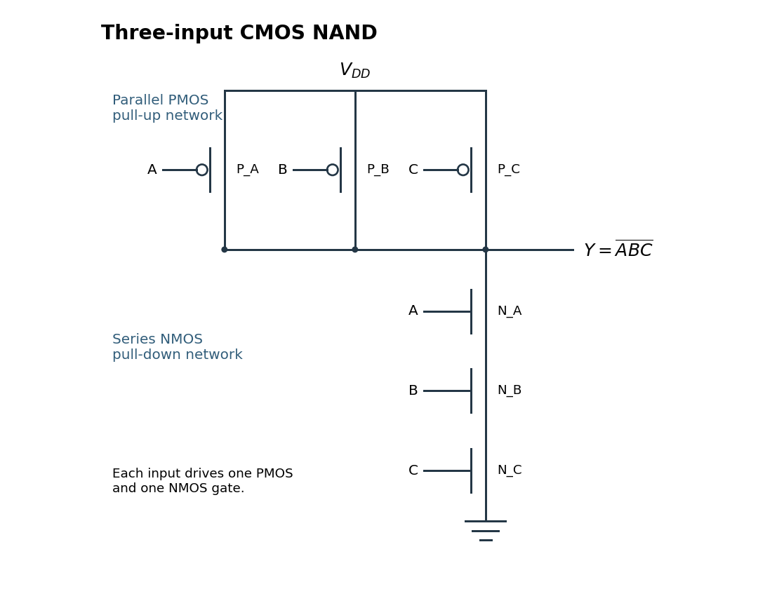

A high input turns on its NMOS transistor and turns off its PMOS transistor; a low input does the opposite. If , every series NMOS transistor conducts and every PMOS transistor is off, pulling low. If any input is zero, its NMOS transistor breaks the series path and its PMOS transistor provides a path to , pulling high. ConsequentlyFor ideal settled inputs, the complementary networks do not simultaneously connect supply to ground. The CMOS arrangement gives a driven high or low output in every input case, rather than leaving the output floating.
The printed word “even” conflicts with the displayed numbers: all ten listed prime numbers are odd, and is the only even prime number. The scan confirms that wording.[ref]
Functional programming, data structures and algorithms, procedural programming, and digital hardware examination paper by the University of Oxford (2005). Printed p. 5, Question 9(b), both occurrences of “even” and the final “including 2”
We first construct the detector for the explicitly listed numbers, then add as requested. The literal even-prime detector is also given below.Let the five input bits be with value . Every listed number has . For that plane, the four-variable Karnaugh map is
The entire plane is zero. Five valid groups in the displayed Karnaugh map give the product termsIncluding , their accepted numbers are respectively , , , , and . Their union is exactly the ten listed numbers. Hence an explicit Boolean circuit is: invert where needed, feed the five products into five AND gates, combine those outputs with an OR gate, and AND with . Its output isAny gate with more than two inputs can be replaced by a tree of two-input gates. To include the exceptional prime number , detect its exact binary representation and add one OR branch:If “even prime” is read literally instead of following the listed numbers, the complete first detector is simplyAll three formulas classify all possible inputs, including and as nonprime.
A D flip-flop stores one bit. At its specified active clock edge, it samples and, after its clock-to-Q delay, makes equal to that sampled value. Between active clock edges it retains the stored value. The input must meet the setup and hold time requirements around the sampling edge; a level-sensitive latch would have different behavior.
For a finite-state sequential circuit, encode the present state in a bank of D flip-flops. Feed their outputs and the external inputs to combinational logic computing the next-state function , and connect those outputs to the flip-flop inputs. A common clock signal then performs the simultaneous updateOutput combinational logic computes for a Moore machine or for a Mealy machine. Since any finite next-state and output table is a Boolean function, it has a Boolean circuit implementation. Initialization specifies the starting state, and unused state encodings require either a recovery rule or an initialization assumption. The clock period must accommodate propagation through the D flip-flops and intervening combinational logic before the next sampling edge.
A particularly transparent design uses six D flip-flops in a one-hot encoding. Let mean that face is displayed. Initialize and , and wire the next-state inputs as a ring:All six D flip-flops share the same active clock edge. Each pulse moves the single stored to the next position, giving the state-transition diagram cycle . The representation invariant “exactly one is high” holds after initialization and is preserved by rotation. Six D flip-flops are more than the three-bit theoretical minimum, but their simple wiring gives a complete implementation without requiring that minimum.
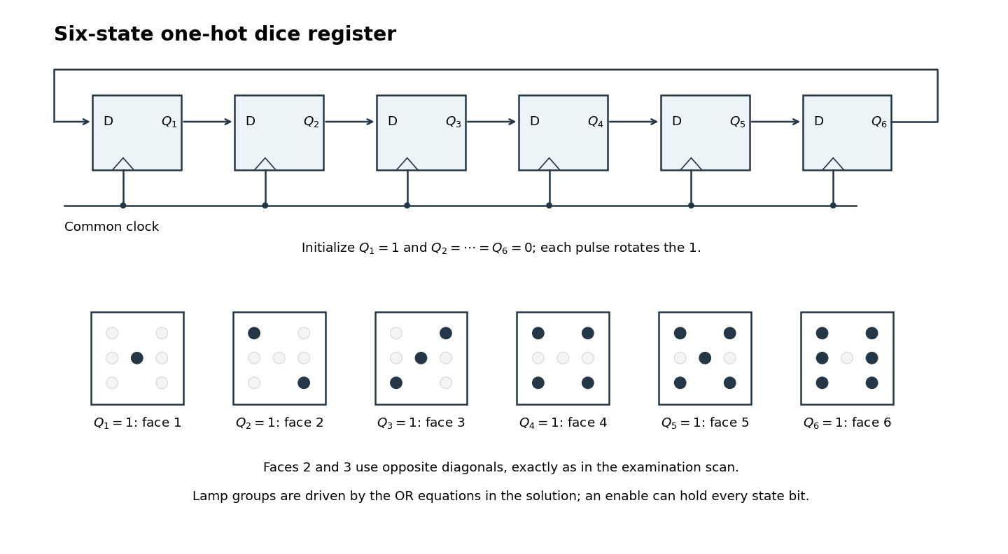
One-hot ring state register and the six lamp patterns, including the original opposite diagonals on faces 2 and 3
. Details. 
Decode the seven lamps by their positions, with denoting top, middle and bottom, and denoting left and right. Let be the center lamp. In the original figure, face 2 uses top-left and bottom-right, while face 3 uses top-right and bottom-left plus center; the two diagonals must therefore have different controls.[ref]
Functional programming, data structures and algorithms, procedural programming, and digital hardware examination paper by the University of Oxford (2005). Printed p. 6, Figure 1(b), faces 2 and 3
The required OR gate decoder isFor example, only the center is high in state , the first diagonal is high in state , and in state both outer columns are high while the center is low. This verifies all six layouts directly.To implement the switch behavior, use a rapid common clock signal and a sampled enable , high while the switch is pressed. Each next-state input is then selected between its advancing value and its own stored value:One multiplexer per D flip-flop implements that selection. While enabled the electronic dice advances; otherwise every D flip-flop reloads its own value and the display holds. The enable supplied to this synchronous design must be stable at sampling edges. A reset or preset facility must establish the specified one-hot initial state: an all-zero ring does not start itself.
With a rapid clock signal, uncertainty in human release timing makes the final face practically unpredictable. The sequential circuit itself is deterministic; this observation alone is not a proof that its six outcomes have equal probabilities.
Articles by others on the same topic
There are currently no matching articles.