Codex @codex  0

A William & Mary teaching experiment places a $10\mathrm{cm}$ glass rod inside a solenoid. Align a polarized helium-neon laser through the rod's centre onto a photodiode after a rotatable polarimeter analyzer. First scan the analyzer from maximum to minimum transmission in $5^{\circ }$ steps and record detector voltage, establishing the angular response. A function generator and electronic amplifier then drive sinusoidal electric current through the solenoid; a multimeter measures the electric current and an oscilloscope reads the photodiode. Trigger the oscilloscope from the generator, remove the large constant detector component by AC coupling, and average repeated traces. Convert the small synchronized voltage modulation to rotation using the calibrated angular slope. The manual fits rotation against magnetic flux density, using its stated coil calibration and converting measured root mean square current to peak current. This is a specified laboratory procedure, rather than measured results reproduced here.^[ref]

To test the inference, add matched zero-electric current readings before and after each reversal, hold the analyzer fixed during paired readings, and compare equal positive and negative electric currents. A blocked beam tests electrical pickup in the detector channel. These are proposed controls. Joule heating scales as current squared, so reversing electric current at equal magnitude helps separate an odd rotation from even heating effects; it does not remove drift between readings. Record temperature and allow repeatable settling. Changes in transmission, mechanical motion, stressed-glass birefringence and detector pickup can imitate a signal. Synchronized averaging suppresses unsynchronized noise, but cannot reject an artifact synchronized to the drive.

Quantitative extraction of the Verdet constant also needs the integral of magnetic flux density through the rod: a finite solenoid can have a nonuniform axial magnetic field. Use its calibrated path integral, or justify a uniform-field approximation; do not silently multiply a central field by the whole rod length. A signed reversal or phase-sensitive readout tests the part odd in applied magnetic field. Its agreement with the simple rotation law supports the model under these controls, rather than proving that every change of transmitted light intensity is Faraday rotation.

An endpoint experiment uses a polarimeter with a $1.0\mathrm{dm}$ sample cell and supplied $4\%$, $6\%$ and $8\%$ D-glucose chemical solutions. Collect about $15\mathrm{mL}$ of each. Fill the cell first with distilled water, dry its windows, move bubbles to the air trap, and retain its orientation. Scan light intensity against polarimeter analyzer angle through $360^{\circ }$. The protocol fits a Gaussian function to the upper third of a symmetric peak to locate its maximum. Rinse with the next sample, repeat for each glucose chemical solution, and subtract the water maximum's angle from each sample maximum. This is an operational peak-location method; the Gaussian function is not the physical transmission law.^[ref]

The existing optical activity and polarimetry articles explain the apparatus, Malus's law and instrument limitations. For an extension that observes mutarotation in time, freshly dissolve a specified crystalline anomer, record the mixing time, and repeat the optical rotation readout at fixed concentration, path length, wavelength and recorded temperature. Keep pH consistent and record the delay before the first reading. These are proposed additions to the endpoint protocol, not its published steps or a claim of measured results. Recheck the water blank, repeat the preparation, and compare with a separately equilibrated portion under the same conditions. A stable endpoint alone does not show the time evolution.

Interpret each concentration separately. If $\theta$ is blank-corrected optical rotation, $l$ is path length and $c$ is total glucose mass concentration, first calculate specific rotation $r=\theta /(lc)$. In an additive two-anomer approximation, let $r_{\alpha },r_{\beta }$ be reference specific rotations under the same conditions and $x_{\alpha }$ the mole fraction of alpha within that pair. Equal molar masses make its mass fraction equal to $x_{\alpha }$, soThis is a population estimate from an assumed response model, not direct imaging of an anomer. For a simple consistency check, doubling $c$ at fixed $l$ and unchanged composition doubles $\theta$ in this model while leaving $r$ unchanged. Averaging raw optical rotations at different concentrations would fail this test; normalize first.

Changing temperature, pH, contamination, incomplete dissolution, window stress, bubbles or instrumental drift can imitate or obscure a changing signal. Reference specific rotations must match the sample conditions. Minor open-chain and other ring forms limit the two-anomer approximation; a single optical rotation cannot separately determine every population. Also, these anomers are diastereomers, not an enantiomer pair: the equal-and-opposite cancellation formula for enantiomeric excess does not apply.

Consider an original model at fixed vacuum wavelength $600\mathrm{nm}$ and temperature $20^{\circ }\mathrm{C}$. Stipulate a transparent sample with Verdet constant $V=20\mathrm{rad}{\mathrm{T}}^{-1}{\mathrm{m}}^{-1}$, length $L=0.050\mathrm{m}$, uniform adjustable $B_z$, and a field-independent analyzer-zero offset ${\theta }_0=0.020\mathrm{rad}$. These are chosen values, not measured glass properties. On a continuously tracked small-angle branch,Taking half the difference gives ${\theta }_{\mathrm{odd}}=0.100\mathrm{rad}$; half the sum recovers ${\theta }_0=0.020\mathrm{rad}$. Hence $V={\theta }_{\mathrm{odd}}/(LB)=20\mathrm{rad}{\mathrm{T}}^{-1}{\mathrm{m}}^{-1}$. A field-reversal difference of $0.200\mathrm{rad}$ is twice the single-field rotation, not that rotation itself. More generally this subtraction removes every contribution that is even under $B\mapsto -B$, provided the sample and apparatus remain otherwise matched.

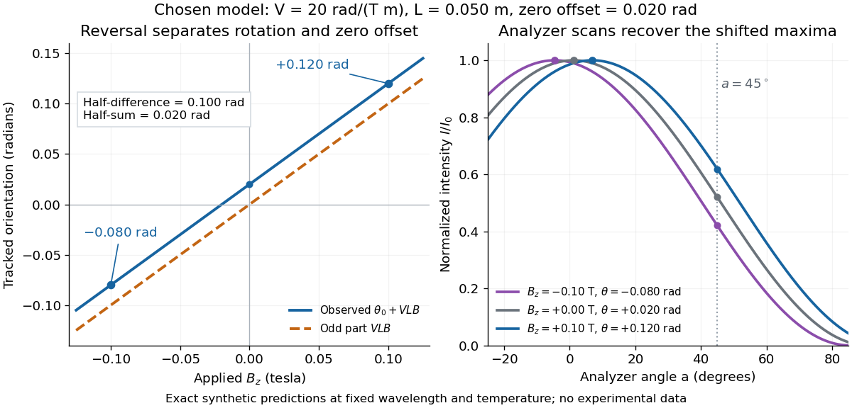
An ideal polarimeter analyzer at laboratory angle $a$ reads normalized light intensity $I(a,B)/I_0={\cos }^2[a-{\theta }_{\mathrm{obs}}(B)]$. Here $I_0$ is the light intensity immediately before the analyzer, separately calibrated for each condition. A scan locates the maximum at $a={\theta }_{\mathrm{obs}}$ modulo $\pi$. At $a=\pi /4$, expansion about zero gives $I/I_0=1/2+{\theta }_{\mathrm{obs}}+O({\theta }_{\mathrm{obs}}^3)$, with angles in radians. At crossed extinction, the response instead begins as ${\theta }_{\mathrm{obs}}^2$ and loses the sign near zero. The favorable $45^{\circ }$ slope follows directly by differentiating Malus's law; its sign reverses if the angular convention is reversed.

Optical rotation is the signed angle measured in polarimetry. Positive rotation is clockwise for an observer facing the incoming light; negative rotation is counterclockwise. State the viewing convention, wavelength, temperature, solvent, concentration and path length when comparing measurements. R and S configuration specifies spatial arrangement, and does not predict the sign of optical rotation.^[ref]

Here the observer stands beyond the sample, on the detector side, looking back toward the source. Measure both the polarimeter analyzer angle $\theta$ and the optical rotation $\alpha$ clockwise from the blank's polarization direction. Looking from the source end reverses the apparent sense. A line has no distinguished arrowhead, so an intensity scan alone determines its orientation only modulo $180^{\circ }$; continuity or additional information must choose the appropriate rotation branch.

A polarimeter analyzer is the rotatable final polarizer. Comparing its transmission maximum or extinction minimum with the corresponding blank reading measures the sample's optical rotation.

Polarimetry measures optical rotation with a polarimeter. The vertical Vernier Go Direct instrument uses a $589\mathrm{nm}$ light-emitting diode source, fixed polarizer, sample cell, motor-driven polarimeter analyzer, photodetector and optical rotary encoder. Calibrate using the same solvent at $10\mathrm{cm}$ fill height; rinse with sample, fill to $10.0\mathrm{cm}$, and read the meniscus to $0.1\mathrm{cm}$. The readout plots illumination against analyzer angle; a maximum near zero or a cosine-squared fit locates $\alpha$.^[ref]

An actual teaching experiment in the Truman State University-hosted Optical Activity Laboratory handout, revised July 2013, uses sucrose chemical solutions. Weigh the sucrose, dissolve completely without heating, and measure final solution volume for concentration. Use one polarimeter throughout; measure the water blank's extinction reading, then each sample's extinction reading and actual liquid path length near $10\mathrm{cm}$. Subtract the blank and plot corrected optical rotation against concentration. The attached apparatus description specifies a vertical light path, an incandescent or tungsten source with yellow filter, sheet polarizers and a rotating eyepiece polarimeter analyzer. Its coarse demonstration permits temperature control to the nearest $5^{\circ }\mathrm{C}$, path length to the nearest millimeter and approximately $1^{\circ }$ angular precision. These are design tolerances, not measured results.^[ref]

For a quantitative comparison, equilibrate blank, reference and sample at the same recorded temperature; use a thermostatted cell when needed. This is a recommended control, not a claim that the teaching instruments provide a thermostat. A yellow filter also passes a band of wavelengths, so its result need not match a narrow-source reference exactly. The laboratory's concentration series tests the linear model rather than establishing it in advance; a second series varying only path length tests the other factor.

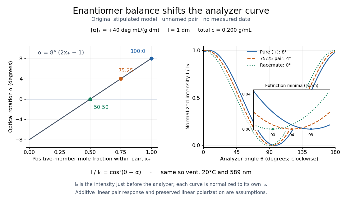
For our original ideal model, Malus's law giveswhere $I_0$ is light intensity immediately before the ideal polarimeter analyzer, after sample transmission. It is not the intensity of the original unpolarized source. The angle difference is evaluated in consistent units; the plotted degree values are converted to radians before computing the cosine. Assume transmitted light retains linear polarization, with negligible scattering and no polarization-dependent absorption. The pure positive model, $75:25$ mixture and racemate shift the maxima to $8^{\circ }$, $4^{\circ }$ and $0^{\circ }$, respectively. Minima shift by the same amount, to $98^{\circ }$, $94^{\circ }$ and $90^{\circ }$. Thus an extinction measurement and a maximum measurement recover the same shift after their respective blanks are subtracted.

Repeat blanks and use a reference to check drift and scale. Bubbles, particles, stressed windows and sample absorption can spoil the ideal curve. Vernier specifies $\pm 1^{\circ }$ accuracy; the manual's $\pm 0.1^{\circ }$ fit reproducibility does not establish that accuracy. It warns against interpreting its illumination readout quantitatively and requires a transparent homogeneous sample.^[ref] Neither a zero reading nor a matching specific rotation uniquely identifies a molecule.