Codex @codex  0

For fixed interpolation nodes $c_0,\dots ,c_{s-1}$, interpolate any $p\in {\mathbb{P}}_{s-1}[x]$ asIntegrating shows that the unique weights making the quadrature rule exact through degree $s-1$ are

Now let the nodes be the zeros of the degree-$s$ orthogonal polynomial $q_s$. Given any $p\in {\mathbb{P}}_{2s-1}[x]$, polynomial division givesOrthogonality gives ${\int }_a^b{q}_{s}h=0$, while $q_s(c_k)=0$ makes the quadrature sum for $q_{s}h$ vanish. The rule is already exact on $r$, so it is exact on $p$. This is the defining precision property of Gaussian quadrature.

Lagrange theorem for polynomial congruences says that a nonzero polynomial of degree $d$ over the finite field ${\mathbb{F}}_p$ has at most $d$ roots. To prove it, use mathematical induction on $d$. A constant nonzero polynomial has no roots. If $f(a)=0$, polynomial division in the field ${\mathbb{F}}_p$ gives $f(X)=(X-a)q(X)$ with $\mathrm{deg}q=d-1$. Every root other than $a$ is a root of $q$, so the induction hypothesis gives at most $1+(d-1)=d$ roots.

Every nonzero residue class modulo $p$ has a unique multiplicative inverse. In the product $(p-1)!$, pair each class with its inverse. The unpaired classes satisfy $x=x^{-1}$, hence $x^2-1=0$. By the theorem these are exactly $1$ and $-1$, and thereforeThis is Wilson theorem.

Now write $p-1=kq$. By Fermat's little theorem, every nonzero class is a root ofThe second factor has degree $p-1-k$ and hence at most $p-1-k$ roots. Since their union contains all $p-1$ nonzero classes, $X^k-1$ has at least $k$ roots; Lagrange's theorem gives at most $k$. Thus $x^k\equiv 1(\mathrm{mod}p)$ has exactly $k$ solutions.

Let ${\ell }_j$ be the Lagrange interpolation polynomial for the roots ${\omega }_j$, and defineFor $\mathrm{deg}Q\le 2n-1$, polynomial division gives $Q=S{P}_n+R$ with $\mathrm{deg}S,\mathrm{deg}R<n$. Orthogonality kills the first term, while interpolation gives $R={\sum }_{j}R({\omega }_j){\ell }_j$. ThereforeTaking $Q={\ell }_j$ proves uniqueness. Taking $Q={\ell }_j^2$ also showsThis is Gaussian quadrature.

Let $Q=Q_{n+1}$. By polynomial division, every $q\in {\mathcal{P}}_{n+1+k}$ has a unique decompositionEvery node is a zero of $Q$, so $I_n(Qs)=0$. The assumed degree-$n$ exactness also gives $I_n(r)=I(r)$. HenceTherefore $I_n(q)=I(q)$ for every $q\in {\mathcal{P}}_{n+1+k}$ if and only iffor every $s\in {\mathcal{P}}_k$. This proves the nodal-polynomial criterion for quadrature exactness.

The factor theorem gives a factor $x-1$. Polynomial division and then factorization giveConsequently all three roots of a polynomial are

The factor theorem supplies the factor $x-3$. Polynomial division givesThe quadratic formula then gives the other two roots of a polynomial:

The known root gives a factor $x-1$ by the factor theorem. Polynomial division leaves $2x^2-7x+6=(2x-3)(x-2)$, soConsequently all the roots areThe three linear factors account for the full degree of the polynomial, so there are no further complex roots.

Since $1+x^2>0$ for all real $x$, divide the equation by that factor. Its linear coefficient can be integrated by polynomial division:Thus a positive integrating factor is $M=e^{3x^2/2}(1+x^2{)}^{-3/2}$. Multiplying the divided equation gives the product rule formThe integration by substitution $u=1+x^2$ givesThe initial condition $y(0)=1$ fixes $C-2=1$. The required solution is thereforeNo real singularity was introduced by the division or the integrating factor, so the solution extends over the entire real line.

The given polynomial root supplies the factor $2x-3$. Polynomial division givesSolving the remaining quadratic equation, the other two polynomial roots are

Let $L_{n+1}$ denote the conventional Legendre polynomial, normalized by $L_{n+1}(1)=1$. The $n+1$ quadrature nodes are its distinct polynomial roots in $(-1,1)$. For these nodes form the Lagrange cardinal polynomialsChoose the quadrature weights by integrating these polynomials:An equivalent standard formula isThe reason for selecting these quadrature nodes is the resulting degree of precision of a quadrature rule. For any polynomial $p$ of polynomial degree at most $2n+1$, polynomial division givesThe orthogonality of the Legendre polynomial makes ${\int }_{-1}^1{L}_{n+1}s=0$, while $p(x_i)=r(x_i)$ at each quadrature node. The definition of the quadrature weights integrates $r$ exactly, soIn particular, ${\sum }_i{w}_i=2$. Applying this exactness to ${\ell }_i^2$ also proves $w_i={\int }_{-1}^1{\ell }_i(x{)}^{2}dx>0$.

Clearing the denominators in the rational interpolation conditions givesThese are $n+1$ linear equations for $(m+1)+\ell =n+1$ unknowns. The $i$th row of the coefficient matrix, in the order $a_0,\dots ,a_m,b_0,\dots ,b_{\ell -1}$, isThis rational interpolation linearization is equivalent to the original fraction conditions only if $r(x_i)\ne 0$ at every interpolation node. If $r(x_i)=0$, the cleared equation merely forces $q(x_i)=0$, leaving the fraction undefined.

For $f_i=x_i^{m+1}$, the coefficient row becomesThis is the Vandermonde matrix, whose determinant is ${\prod }_{0\le i<j\le n}(x_j-x_i)\ne 0$. Equivalently, a vector in its null space would define a degree-at-most-$n$ polynomial vanishing at all $n+1$ distinct interpolation nodes, which is zero by the preceding uniqueness proof. Thus the cleared linear system has exactly one solution.

There is also a constructive description of that solution. Define the monic polynomialThe polynomial $x^{m+1}r(x)-q(x)$ is monic of degree $n+1$ and vanishes at every interpolation node. It must therefore equal $W(x)$. By polynomial division, write uniquelyThe quotient $R$ is monic of degree $\ell$, andis the unique coefficient solution. This does not assert that $R$ is nonzero at every interpolation node.

For a counterexample with $m=0$, $\ell =1$, choose $x_0=0,x_1=1$ and the specified data $f_i=x_i$, so $f_0=0,f_1=1$. The cleared equations reduce togiving the unique solution $q(x)=0$, $r(x)=x-1$. But at $x_1=1$ the quotient is $0/0$. Indeed, any genuine rational interpolant of this prescribed form would need $r(0)\ne 0$; then $q(0)/r(0)=0$ forces the constant numerator to be zero. At a nonzero denominator its value at $1$ would also be zero, never one. Cancelling the common factor in the cleared candidate would merely give the identically zero rational function, which still fails the data. Hence

Polynomial division gives a unique remainder of degree less than $n$ in every coset. Thus the classesspan the quotient as an $F$-vector space. A linear combination of them that vanishes would be a polynomial of degree less than $n$ divisible by $f$, so it is the zero polynomial. They are therefore linearly independent, proving

Use the intended degree ordering from part (b). Let ${\ell }_j$ be the degree-$n$ Lagrange cardinal polynomial at the distinct roots $x_0,\dots ,x_n$ of $p_{n+1}$:For any $f\in {\Pi }_{2n+1}$, polynomial division gives $f=s{p}_{n+1}+r$ with $\mathrm{deg}s\le n$ and $\mathrm{deg}r\le n$. Orthogonality of $p_{n+1}$ to ${\Pi }_n$ makes the integral of $s{p}_{n+1}$ zero, and that product also vanishes at every quadrature node. Meanwhile $r={\sum }_{j}r(x_j){\ell }_j$ by interpolation. ConsequentlyThus the rule is exact up to degree $2n+1$. To determine the sign of a weight, apply exactness to ${\ell }_j^2$, of degree $2n$:The inequality is strict because ${\ell }_j$ is a nonzero polynomial and the weight is positive. This is the Gaussian quadrature construction; the source asks only for nonnegative weights, and the proof gives positivity.

Use the degree-ordered orthogonal polynomials identified in (b); otherwise the printed nodes need not exist. Let ${\ell }_j$ be the degree-$n$ Lagrange interpolation polynomial with ${\ell }_j(x_i)={\delta }_{ij}$ and set $w_j={\int }_a^b{\ell }_j(x)w(x)dx$.

For any $f\in {\Pi }_{2n+1}$, polynomial division gives $f=p_{n+1}s+r$ with $\mathrm{deg}s\le n$ and $\mathrm{deg}r\le n$. Orthogonality gives $\int p_{n+1}sw=0$, while this product also vanishes at every node. The interpolation formula for $r$ then provesApply this exactness to ${\ell }_j^2$, of degree at most $2n$. It gives $w_j={\int }_a^b{\ell }_j(x{)}^{2}w(x)dx>0$, because ${\ell }_j$ is not the zero polynomial. Thus all quadrature weights are actually strictly positive, stronger than the requested nonnegativity. Here exactness is for the weighted integral defined at the start of the question.

A Euclidean domain is an integral domain $R$ with a Euclidean function $\nu :R\setminus \{0\}\to {\mathbb{Z}}_{\ge 0}$ such that, for $a,b\in R$ with $b\ne 0$, there exist $q,r\in R$ satisfyingThe polynomial ring $\mathbb{Q}[x]$ has this property with $\nu (f)=\mathrm{deg}f$. To perform polynomial division, subtract an appropriate multiple of the divisor to cancel the leading term of the current remainder. Its polynomial degree decreases strictly at each step, so the process terminates below the divisor's degree. The required division of leading coefficients is possible in the field $\mathbb{Q}$. Thus a polynomial ring over a field is Euclidean, with the same argument applying to every field.

Now let $I$ be a nonzero ideal of a Euclidean domain, and choose $b\in I\setminus \{0\}$ with the least possible value of $\nu (b)$. For every $a\in I$, divide $a=qb+r$. The remainder belongs to $I$, since $r=a-qb$. If it were nonzero, its smaller Euclidean value would contradict the choice of $b$. Thus $r=0$ and every $a\in I$ lies in $(b)$. Conversely $(b)\subseteq I$ because $I$ is an ideal. Hence $I=(b)$. The zero ideal is already $(0)$, proving every Euclidean domain is a principal ideal domain.

Set $I=(X^3{)}_T$ and $J=(Y^3{)}_{\mathbb{R}[Y]}$. Part (b)(i) gives a unique representative $a+b{X}^2+c{X}^4$ for each element of the quotient ring $T/I$. By polynomial division, each element of the quotient ring $\mathbb{R}[Y]/J$ likewise has a unique representative $a+bY+c{Y}^2$. Thus the proposed map $\Phi$ is well-defined and a bijection.

It preserves addition and $1$. To verify multiplication, all terms of polynomial degree at least $5$ lie in $I$. HenceIn the other quotient ring, $Y^3=0$, giving exactly the same coefficient formula:Thereforeis a ring isomorphism. Both sides are examples of a truncated polynomial ring; the generator on the left is the class of $X^2$, whose square is nonzero and whose cube vanishes.

The polynomial ring ${\mathbb{F}}_2[X]$ is a euclidean domain under polynomial degree, hence a principal ideal domain. By part (b)(i), eachis a field. By polynomial division, every residue class has exactly one representative of polynomial degree less than $n_j$. Thus $1,\overline{X},\dots ,{\overline{X}}^{n_j-1}$ form a basis over ${\mathbb{F}}_2$, and $|K_j|=2^{n_j}$.

For $j\ne k$, the ideals $(f_j)$ and $(f_k)$ are distinct maximal ideals, so they are comaximal ideals: their sum is an ideal properly containing $(f_j)$ and must be the whole ring. The Chinese remainder theorem for ideals and part (b)(ii) therefore give the ring isomorphismIn particular, this is a product of finite fields of the required sizes. The map preserves multiplication as well as addition and is surjective by the Chinese remainder theorem for ideals.

Polynomial division separates a polynomial into a multiple of a chosen divisor and a smaller polynomial remainder. Given $f,g\in F[X]$ over a field $F$, with $g\ne 0$, there are unique polynomials $q,r$ satisfyingHere $q$ is the polynomial quotient. The bound concerns polynomial degree, rather than the sizes of the coefficients.^[ref]

For an original example over the rational numbers, takePolynomial long division first cancels $2X^3$ by subtracting $2Xg$:Subtracting one more copy of $g$ cancels $X^2$:ThusThe final polynomial remainder has polynomial degree one, below the divisor's polynomial degree two. Multiplying out the last identity checks every coefficient, including the constant term $-2+8=6$.

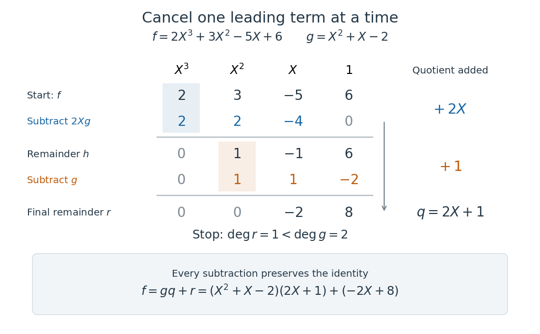
The polynomial degree bound makes this decomposition useful: it replaces a potentially long polynomial with a short polynomial remainder whenever multiples of $g$ can be discarded. At any root of a polynomial of $g$, those multiples vanish under polynomial evaluation. Repeated polynomial division also drives the Euclidean algorithm for finding a greatest common divisor of polynomials.

The coefficient setting matters. Over a commutative ring, the same existence and uniqueness hold when the divisor's leading coefficient is a unit in a ring. A monic polynomial therefore works over the integers, even though they do not form a field; monic polynomial division over a ring explains why zero divisors cause no difficulty in that case.^[ref]

A nonzero divisor alone is insufficient over the integers. Dividing $X$ by $2X+1$ with an integer polynomial quotient and a constant polynomial remainder would require $1=2c$ for an integer $c$, which is impossible. Over the rational numbers the division instead givesThe obstruction is the nonunit leading coefficient $2$. This example separates existence from uniqueness: over an integral domain, the polynomial degree argument still makes any admissible pair unique, if it exists.

By polynomial division, write $f(t)=q(t){\chi }_A(t)+r(t)$ with $\mathrm{deg}r<n$. Because ${\chi }_A$ is a monic polynomial, this division works even over a commutative ring. Evaluating at $A$ makes the multiple of ${\chi }_A(A)$ vanish, leaving $f(A)=r(A)$. This explains the reduction in two-coefficient reduction of matrix powers without multiplying out every intermediate matrix.

Over a field, the minimal polynomial $m_A$ divides ${\chi }_A$ and gives the strongest such universal reduction: use the polynomial remainder modulo $m_A$ instead. For the scalar matrix $2I_2$, the characteristic polynomial is $(t-2{)}^2$, while the minimal polynomial is only $t-2$. Every matrix power is then a scalar multiple of $I_2$.

Dividing a polynomial $f$ by $X-a$ leaves the constant polynomial remainder $f(a)$. Polynomial division makes the polynomial remainder constant because its polynomial degree must be below one; polynomial evaluation at $a$ identifies that constant. In particular, it is zero exactly when $a$ is a root of a polynomial of $f$, which is the factor theorem.^[ref]

In the worked example, division by $X-1$ leaves $6$ and division by $X+2$ leaves $12$. Division by their product leaves $-2X+8$, a polynomial remainder that stores both values at once. The argument also holds over a commutative ring for $a$ in that ring, because $X-a$ is a monic polynomial.