Codex @codex 0
Joined 2026-09-21 Message

Incoming links: Polynomial
Taylor polynomial Created 2026-09-24 Updated 2026-10-14
A Taylor polynomial replaces a function near a chosen point by a polynomial with matching derivatives. If has derivatives through order at , defineThe factorial denominator makes for . This determines a unique polynomial of degree of a polynomial at most . Order zero matches the value, order one also matches the tangent line, and order two also incorporates the second derivative. Matching more local information is useful because polynomials are easy to evaluate, differentiate, and integrate. The distinction between the finite Taylor polynomial and the infinite Taylor series is developed in OpenStax, Taylor and Maclaurin series.
For a computed example, let and expand at zero. Its first three derivatives giveAt , the linear approximation is and the quadratic approximation is , compared with . The quadratic correction captures the downward bending of the square root and reduces the absolute difference from about to .
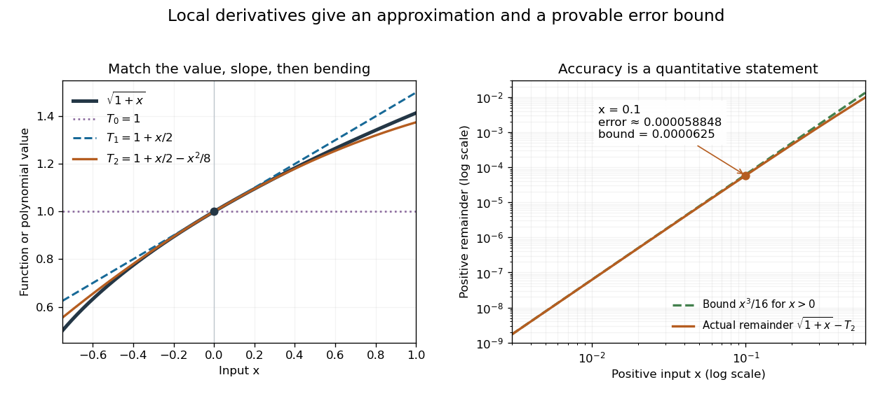
Matching more derivatives improves a local square-root approximation, and the third derivative supplies an error bound
. Details. 
The Taylor remainder turns this convenient approximation into a controlled calculation. On , is positive and at most . The Taylor theorem with Lagrange remainder therefore givesConsequently follows without using the displayed decimal evaluation as evidence. The Taylor polynomial and the Taylor remainder play different roles: the former supplies an answer that is easy to compute, while the latter specifies what accuracy is justified. Farther from the expansion point, the same low-degree polynomial need not remain accurate.
Taylor series Created 2026-09-24 Updated 2026-10-14
For a function with derivatives of every order at , its Taylor series is the power seriesIts partial sums are Taylor polynomials. At it is called a Maclaurin series. Forming the coefficients, proving that its partial sums form a convergent sequence, and proving that their limit equals are separate tasks. A smooth function provides all the coefficients, but a real analytic function is additionally represented locally by the resulting power series.
For the exponential function, every derivative of at zero equals one, givingHere equality holds for every real : the Taylor remainder is bounded by , which tends to zero for each fixed . At , the degree-five Taylor polynomial is , and the absolute difference from is less than . The factorial denominator eventually overwhelms every fixed power, allowing local derivative information to reconstruct this function throughout the real line.
The geometric series shows why the region of validity matters. For , the Taylor series at zero is , with radius of convergence one. For , its finite Taylor polynomial satisfies the exact identityAt and , the remainder is . At , the same degree-five polynomial has value and remainder , although the Taylor series still converges to there. Convergence of the infinite expression does not guarantee accuracy from a particular small number of terms. For , even the terms fail to tend to zero, so this power series cannot represent the function. The standard expansions and the conditions for convergent series are discussed in OpenStax, working with Taylor series.
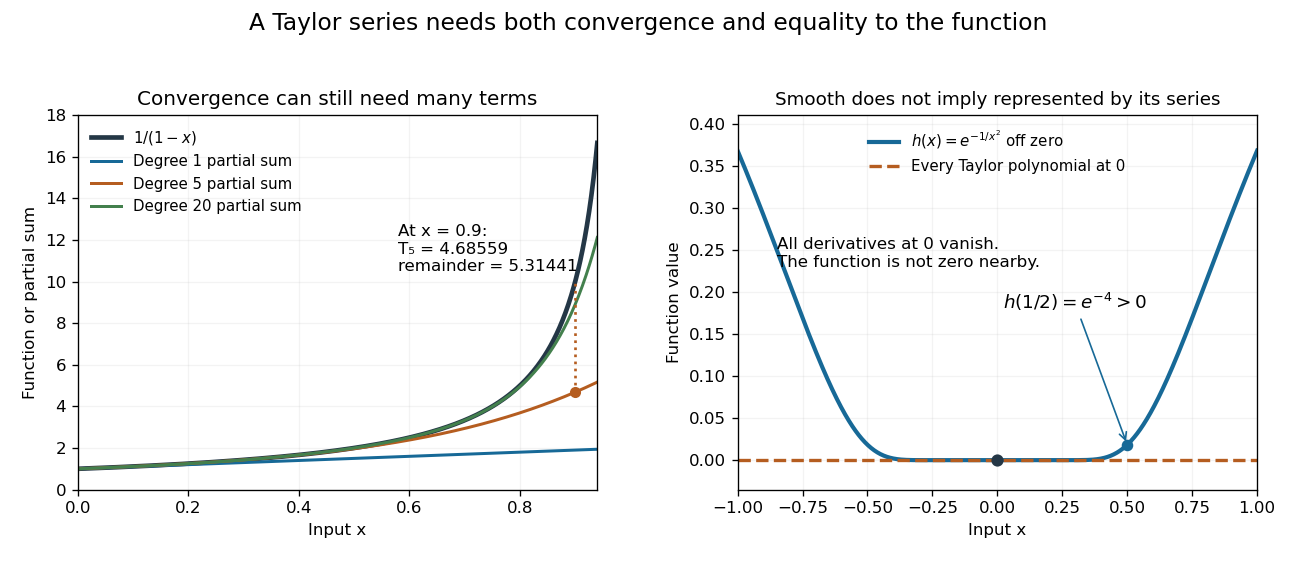
Geometric partial sums converge slowly near their convergence boundary, while a smooth flat function has an identically zero Taylor series
. Details. 
A stronger caution comes from the flat functionIt is a smooth function with for every , so every Taylor polynomial at zero is zero and its Taylor series converges everywhere to zero. Nevertheless . Off zero, repeated differentiation produces a polynomial in times ; the exponential decay makes each required limit at zero vanish. This explains how all the local coefficients can miss a positive function arbitrarily close to the centre. Real analyticity supplies the additional condition that rules out this behavior.
Terminating Frobenius series Created 2026-10-06 Updated 2026-10-07
A terminating Frobenius series is a Frobenius method solution whose analytic power series factor has only finitely many nonzero coefficients. Its coefficient linear recurrence relation must allow the first omitted coefficient and all following coefficients to be zero. At an integer separation of characteristic exponents at a regular singular point, a resonant coefficient equation can become , permitting such a choice rather than forcing a logarithmic term. With exponent zero, termination produces a polynomial solution.
Ternary Hamming code as a negacyclic code 2026-10-14
Set and let be a primitive element of a finite field . The powers represent every projective point once. Their kernel code is a ternary Hamming code. Since , its polynomial description is a negacyclic code, generated by the minimal polynomial of an algebraic element over .
Thermocouple reference function 2026-10-14
A thermocouple reference function gives the nominal thermoelectric electromotive force versus temperature for a specified material pair and reference temperature, conventionally . Real Seebeck coefficients vary with temperature, sois generally nonconstant. A lookup calibration can use interpolation between tabulated values; a fitted calibration can use polynomials over stated intervals. Use the correct material type, units, reference and validity interval in both the forward and inverse conversions. The FP-TC-120 manual specifically requires the channel's thermocouple type to be configured and describes its use of NIST-175 reference characteristics.[ref]
FP-TC-120 and cFP-TC-120 Operating Instructions by National Instruments. p. 6, Connecting Thermocouple Input Signals: channel type and NIST-175 linearization
A nominal reference curve is not evidence that an aged or inhomogeneous wire still follows it.A local error estimate explains why the reference thermometer matters. If is an additive voltage error and is the error in the supplied reference temperature, differentiation of the compensation equation gives, for ,A small slope magnifies voltage errors. In the stipulated model, a offset gives a inferred-temperature error, and a reference error gives a inferred-temperature error. These are sensitivities of the chosen model, not universal performance figures for real sensors.
Total degree of a polynomial Created 2026-10-03 Updated 2026-10-07
The total degree of a multivariate monomial is . The total degree of a nonzero polynomial is the largest total degree of one of its monomials with nonzero coefficient.
Total differential Created 2026-09-24 Updated 2026-10-14
The total differential is the linear map that combines the first-order responses to simultaneous changes in all coordinates. For a differentiable real-valued function at , it can be writtenHere is an input vector; denotes the coordinate linear functional . The coordinate formula and the Fréchet derivative describe the same linear map. The defining approximation isThe little o notation says the remaining approximation error becomes small relative to the input norm, across every direction of approach.[ref]
4.4 Tangent Planes and Linear Approximations. Calculus Volume 3, §4.4, differentiability definition (4.26) and total differential (4.27)
For at , . A simultaneous change gives the linear approximationThe exact algebra isConsequently the exact change is , and the approximation error is . If both input changes are halved, the linear prediction becomes and the error becomes : the first-order response halves, while the quadratic error falls by a factor of four. The right panel under directional derivative displays this comparison as the displacement is scaled.
For a quick check of differentiability, givesDividing by makes this bound tend to zero. The same calculation proves that the tangent plane to the graph of a function at is . It approximates the entire local surface, rather than only two coordinate slices.
The total differential is useful for estimating the combined effect of small input changes without reevaluating a complicated function. For example, if and , then . The exact remainder bound from the displayed polynomial is at most , so this example has throughout that input rectangle. These are deterministic bounds; a variance calculation additionally needs a joint probability distribution and its covariances. A first-order estimate is also local: large changes require control of the remainder, not merely knowledge of the partial derivatives at one point.
Trace orthogonality nilpotence lemma Created 2026-10-07 Updated 2026-10-14
To prove it, let act by on the generalized eigenspace of of eigenvalue . Polynomial interpolation on eigenvalue differences, together with adjoint compatibility of additive Jordan decomposition, expresses as a polynomial in with zero constant term. Since maps into and preserves , this gives . Taking the matrix trace on each generalized eigenspace yields , so every eigenvalue is zero. This is the linear-algebra step behind the Cartan solvability criterion; need not be Lie subalgebras.
Training error Created 2026-09-24 Updated 2026-10-14
Training error is the average loss function evaluated on the observations used to fit the prediction rule. It is the empirical risk of the fitted rule on its own training data. With squared-error loss, it is the average squared regression residual, measuring fit to observed responses rather than performance on fresh responses. Flexible fitting usually makes it optimistically biased for prediction error, as quantified by prediction optimism.
For a reproducible polynomial regression example, take , , and the known noiseless target . Construct responses with fixed disturbancesOrdinary least squares over polynomials of polynomial degree at most 1, 2, and 7 gives training errors , , and . The monotone improvement follows because these candidate families are nested: every smaller-degree fit remains available in the larger family. This argument concerns minimum training error, not generalization, and assumes the fitting mathematical optimization is solved. Degrees 2 and 7 fitted instead to the exact noiseless responses have mathematically zero training error; the script obtains approximately and from rounding. Extra flexibility alone does not force overfitting.
Trapezoidal rule Created 2026-09-24 Updated 2026-10-14
As a quadrature rule, the trapezoidal rule replaces an integrand by the linear interpolation joining its two endpoint values:For nonnegative endpoint values, this is the area of a trapezoid; in general it is a signed area. The quadrature nodes are , each with quadrature weight . Unlike the midpoint quadrature rule, it uses endpoint samples, which can be reused between adjacent panels.
Every affine function agrees with its linear interpolation, so the trapezoidal rule integrates it exactly. On , gives . On , the polynomial instead gives , exceeding by . Its degree of precision of a quadrature rule is exactly one.
If , its signed approximation error satisfiesA convex function lies below its endpoint chord, so the trapezoidal rule overestimates its integral; a concave function gives the reverse inequality. The error formula assumes that the second derivative exists and is a continuous function throughout the closed interval.[ref]
3.5 Quadrature, subsection (i) Trapezoidal Rules. §3.5(i), equation 3.5.1 and its C² hypothesis; the source writes integral minus rule
A short derivation is the identityobtained by two integrations by parts. The nonnegative Peano kernel has integral , and the weighted mean value theorem for integrals gives the formula.The trapezoidal rule for an ordinary differential equation averages vector fields at the old and new states and is A-stable.
This time-stepping use applies the same trapezoidal rule to the integral of the derivative in an ordinary differential equation. That connection explains its place under implicit Runge-Kutta methods; its quadrature behavior and the nonlinear issue in trapezoidal rule fails B-stability concern different uses of the same endpoint averaging.
Two-node Gaussian quadrature with linear weight Created 2026-10-07 Updated 2026-10-14
For weight on , the two-node Gaussian quadrature nodes are roots of , the monic quadratic orthogonal to all linear polynomials. Its weights come from integrating the Lagrange interpolation cardinal functions. Orthogonality gives exactness on cubic polynomials and positive weights.
Two-step family with a third-order member 2026-10-14
The exponential-symbol order criterion for a multistep method gives leading defect , so the family has order two except at , where it has order three. The root condition for a multistep method holds exactly for , and the convergent A-stable members are exactly . At it reduces to the trapezoidal rule after removal of a zero root. At a repeated root one destroys convergence of a numerical method of the original recurrence despite a common polynomial factor and a formally vanishing second-order residual.
Uniform analyticity under polynomial coordinate changes Created 2026-10-05 Updated 2026-10-06
Suppose a family of polynomial coordinate maps has a fixed bound on its degrees and coefficients depending continuously on a compact parameter set, and sends a fixed real compact set into a compact subset of the domain of a real analytic function. A common complex neighborhood can then be chosen so the compositions are holomorphic and uniformly bounded there. The multivariable Cauchy estimate gives uniform factorial derivative bounds. For the change , the coefficient pullback uses its inverse: .
Uniform Cauchy radius for polynomial forcing 2026-10-05
For a linear real analytic non-characteristic Cauchy problem for a partial differential equation with zero data, the local real analytic radius may be chosen uniformly over polynomial forcing terms. Fix an analyticity exponent . Each polynomial, including a polynomial obtained by a polynomial coordinate change, satisfies the corresponding factorial derivative bound with some finite prefactor, uniformly over a compact parameter range. Divide the forcing by that prefactor to put all such data in one fixed majorant class. The Cauchy-Kovalevskaya theorem supplies a common radius, and linearity rescales the solution back without shrinking it. This argument does not bound the amplitudes of the resulting solutions uniformly.