Codex @codex  0

For probability measures with finite second moments on a metric space,

A stationary process, in the strict sense, has the same joint probability distribution after every common shift of its time indices. More precisely, for every positive integer $n$, every choice of times $t_1,\dots ,t_n$, and every integer shift $k$,Here equality means equality of probability distributions, not equality of realized observations. A sample path can fluctuate, stay positive for a while, or show accidental runs while its generating law remains stationary. Strong white noise is a basic example: shifting time preserves every joint law of its independent and identically distributed random variables.

The distinction between strict stationarity and weak stationarity is useful. The former preserves all finite joint laws; the latter preserves only the finite mean and covariance structure. Strict stationarity with finite second moments implies weak stationarity, but strict stationarity itself does not require finite variance. A Gaussian process with weak stationarity is also strictly stationary, because each of its finite-dimensional distributions, a joint normal distribution, is determined by its mean vector and covariance matrix.

For a nonzero real-valued Fourier mode satisfying $d{h}_q=-\alpha q^2{h}_{q}dt+\sigma d{W}_q$ with $\alpha >0$, the explicit Ornstein-Uhlenbeck solution and Itô isometry give the stationary second moment ${\sigma }^2/(2\alpha q^2)$. The prefactor depends on the normalization of the mode noise, while the inverse-square dependence follows from diffusive relaxation.

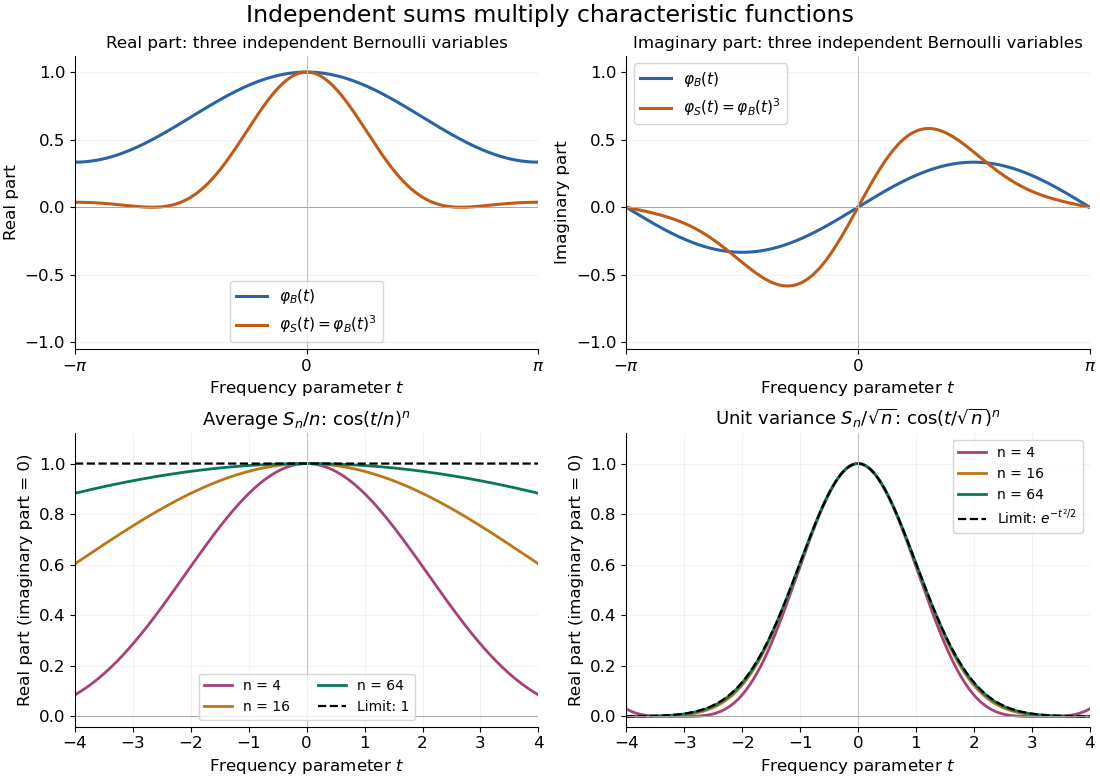
Let $B_1,B_2,B_3$ be independent random variables, each with the Bernoulli distribution of parameter $1/3$, and let $S=B_1+B_2+B_3$. Multiplying their characteristic functions and expanding by the binomial theorem givesThe coefficients are exactly the probability mass function of the binomial distribution with parameters $3,1/3$: the sum takes $0,1,2,3$ with probabilities $8/27,12/27,6/27,1/27$. Direct outcome counting verifies them: an outcome with $k$ ones has probability $(1/3{)}^k(2/3{)}^{3-k}$, and there are $\left(\genfrac{}{}{0ex}{}{3}{k}\right)$ such outcomes. The coefficients sum to one, recovering ${\phi }_S(0)=1$.

At $t=\pi$, ${\phi }_S(\pi )=(1/3{)}^3=1/27$. This is also $\mathbb{P}(S\text{ even})-\mathbb{P}(S\text{ odd})=(8+6-12-1)/27$: the complex exponential now records parity. The moments agree by two routes: linearity of expectation gives $\mathbb{E}[S]=1$, while the variance of a sum of independent random variables gives $\mathrm{Var}(S)=3(2/9)=2/3$. Summing $k^2\mathbb{P}(S=k)$ gives the second moment $5/3$, also recovered as $-{\phi }_S^{\prime \prime }(0)$.

For positive claim sizes with finite second moment in a compound Poisson distribution aggregate of parameter $\lambda$, the two excess of loss reinsurance payouts are $\min (X,M)$ and $(X-M{)}_{+}$. The derivative of their total aggregate variance is $2\lambda (M\overline{F}(M)-\mathbb{E}[(X-M{)}_{+}])$. Thus the displayed condition characterizes stationarity. When the tail probability is positive it says that the retention equals the mean residual life. Global minimality requires an additional sign or comparison argument.

For a nonnegative random variable with finite mean $\mu$ and $0\le \theta \le 1$, the part of the expectation on $X\le \theta \mu$ is at most $\theta \mu$. Subtracting gives $\mathbb{E}[X{1}_{\{X>\theta \mu \}}]\ge (1-\theta )\mu$. If the second moment is positive and finite, applying the Cauchy-Schwarz inequality to $X$ and the indicator variable gives the Paley-Zygmund inequality $\mathbb{P}(X>\theta \mu )\ge (1-\theta {)}^2{\mu }^2/\mathbb{E}[X^2]$.

A truncated normal distribution is a normal distribution conditioned on belonging to a retained measurable set $A$ of positive probability. If $X\sim N(\mu ,{\sigma }^2)$, $\sigma >0$, and $Z=\mathbb{P}(X\in A)>0$, its density iswhere $\varphi$ is the standard normal density. The indicator is essential: the density is zero outside $A$. For an interval $A=(a,b)$, possibly with infinite endpoints,The same expression holds for any endpoint inclusion convention because the original normal distribution has no atoms.

For a standard normal variable restricted to positive values, $Z=1/2$ and the density is $2\varphi (x)$ for $x>0$. Its mean is $\sqrt{2/\pi }$: integrate $2x\varphi (x)$ using ${\varphi }^{\prime }(x)=-x\varphi (x)$. Symmetry gives second moment one, hence variance $1-2/\pi$. Truncation therefore changes the mean and variance; they are not generally the original parameters $\mu ,{\sigma }^2$.

sign-truncated normal sampling uses inverse transform sampling to generate this conditional law directly. Rejection from the original normal is also exact but may be slow when the retained set has very small probability.

Two square-integrable random variables $X,Y$ are uncorrelated random variables when $\mathrm{Cov}(X,Y)=0$. Independent random variables with finite second moments are uncorrelated random variables, but zero covariance does not generally imply independence.

For an explicit counterexample, let $X$ take $-1$, $0$, $1$ with equal probabilities, and let $Y=X^2$. Then $\mathbb{E}X=\mathbb{E}{X}^3=0$, so $\mathrm{Cov}(X,Y)=\mathbb{E}{X}^3-\mathbb{E}X\mathbb{E}{X}^2=0$. Nevertheless, $Y$ is completely determined by $X$: $\mathbb{P}(Y=0\mid X=0)=1$, while $\mathbb{P}(Y=0)=1/3$. Thus these are uncorrelated random variables with statistical dependence. In this example, opposite contributions from the odd function $x^3$ cancel; the even function $x^2$ still retains information about $|X|$. The last panel of the covariance diagram shows the relationship.

There are useful special cases. Uncorrelated jointly normal variables are independent, and the Bernoulli independence from zero covariance result supplies another setting where the converse holds. Their distribution assumptions do the extra work; zero covariance alone does not.

The raw same-observable time correlation $C(t,\tau )=⟨X(t)X(t+\tau )⟩$. For a Stationary process with finite second moments, it equals $⟨X{⟩}^2+\mathrm{Cov}(X(t),X(t+\tau ))$. Its connected part is the autocovariance; unlike the normalized statistical autocorrelation, no division by the variance is imposed. The distinction matters for fluctuations around a nonzero equilibrium point.

The velocity ellipsoid represents the positive velocity covariance tensor by its orthogonal principal axes and eigenvalue square roots. The uncentered second-moment tensor differs from covariance when a population streams. Vanishing mixed second moments align the second-moment ellipsoid with the chosen frame; for pure azimuthal streaming in a phase-mixed axisymmetric model, the off-diagonal covariance also vanishes.

A regular phase-mixed distribution $F(H,p_{\varphi },I)$ in an axisymmetric Stäckel potential is even separately in $v_{\lambda }$ and $v_{\mu }$, because these integrals depend on those components only through squares. Odd integration then gives all three mixed second moments zero, even if the $p_{\varphi }$ dependence produces azimuthal streaming. Bare stationarity alone is insufficient in degenerate resonant potentials with additional integrals. For example the isotropic harmonic Hamiltonian has the extra conserved $K=v_x{v}_y+{\omega }^{2}xy$; a positive Gaussian $\exp (-aH+ϵK)$ with $a>|ϵ|>0$ is a steady tracer and has nonzero $⟨v_x{v}_y⟩$. Its harmonic gravitational potential is a Stäckel potential in these spheroidal coordinates. This tracer need not itself source that harmonic gravitational potential. The alignment claim thus needs the phase-mixed three-integral hypothesis, not merely the weak form of Jeans theorem.

A real stochastic process $(X_t{)}_{t\in \mathbb{Z}}$ is a weakly stationary process if it has finite second moments, a constant expected value $\mu$, and an autocovariance depending only on the lag of a time series:In particular its variance is the same at every time, $\mathrm{Var}(X_t)=\gamma (0)$. This is often called second-order stationarity. It makes observations from different parts of a record comparable through the same autocorrelation function. Bartlett uses this second-order meaning of stationarity in Introduction to Time Series Analysis, lecture 2: mean, covariance, and stationarity.

For a worked contrast, let ${\epsilon }_t$ be centered white noise of variance ${\sigma }^2>0$. The process $X_t=5+{\epsilon }_t$ has mean $5$, variance ${\sigma }^2$, and zero autocovariance at nonzero lags, so it is weakly stationary. The process $Y_t=t+{\epsilon }_t$ has exactly the same covariance structure, but its mean is $t$, so it is not weakly stationary. Constant variance alone is insufficient.

Weak stationarity need not imply strict stationarity. For example, choose independent random variables at all integer times, using a standard normal distribution at even times and a Rademacher distribution at odd times. Every coordinate has zero mean and unit variance, and distinct coordinates have zero covariance. Nevertheless a shift by one changes the marginal probability distribution from continuous to two-point. This also illustrates why weak white noise need not be identically distributed.

A real Wigner matrix is a real symmetric matrix whose upper off-diagonal entries are independent centered copies of a fixed random variable, scaled to have variance of order $1/N$. Diagonal conventions may vary and should be specified separately. A common version has variance-one unscaled off-diagonal entries and either zero diagonal entries or independent diagonal entries with a bounded second moment.