Codex @codex  0

Total harmonic distortion measures the root-sum-square amplitude of the selected higher harmonic components relative to the fundamental amplitude. For nonzero $A_1$ and one common amplitude convention,Peak amplitudes or root mean square amplitudes give the same ratio when used consistently for all sinusoids. The finite upper order $M$, measurement bandwidth, and treatment of noise must be specified. The primary Anritsu procedure distinguishes this fundamental-normalized definition from normalization by the full harmonic component sum.^[ref]

For an original example, let a waveform have fundamental peak amplitude $2\mathrm{V}$, second harmonic component $0.06\mathrm{V}$, and third harmonic component $0.08\mathrm{V}$, with no other components. ThenA logarithmic amplitude-ratio report is $20{\log }_{10}(0.05)\approx -26.02\mathrm{dB}$. The phases do not enter this RMS sum because distinct integer harmonic components are orthogonal over a full period.

If the denominator instead includes the fundamental and all included harmonic components, excluding DC, the resulting ratio isabout $4.994\%$ in the example. The two conventions are close at low distortion but differ markedly when higher harmonic components are large; only the latter is bounded by one. A quoted percentage without its denominator convention is incomplete. Broadband noise is a different contribution and is not silently included in the displayed THD formula.

A motivating apparatus uses a clean sinusoidal source, the device under test, and calibrated receivers tuned to the fundamental and harmonic component frequencies. Anritsu's worked system calibrates the receiver over those frequencies before combining separate measurements.^[ref] With an FFT-based instrument, spectral leakage bias in harmonic distortion measurements can misassign a strong fundamental to harmonic component bins; aliasing and insufficient receiver bandwidth can also hide or relocate components. Small THD therefore describes a stated test and analysis, not every possible waveform or operating level.

A transfer function packages the response of a linear time-invariant system into a rule for turning a plant input into a plant output. Instead of solving a differential equation separately for every signal, take a Laplace transform, multiply by $G(s)$, then transform back. This also makes it possible to compare slow and fast oscillations through the continuous-time frequency response.

Here consider a continuous-time, causal, finite-dimensional linear time-invariant system with one plant input $u(t)$ and one plant output $y(t)$. With every initial state set to zero, its transfer function is defined byThe ratio $G(s)=Y(s)/U(s)$ is used where $U(s)\ne 0$ in a common Laplace convergence region; $G$ describes the system, independently of that particular plant input. Zero initial state matters: stored motion or another nonzero initial condition can contribute to the plant output even when the plant input vanishes. ^[ref]

The first-order low-pass filter below shows the same transfer function predicting both a step and a sustained sinusoid. Its pole gives a decay rate, its value at zero gives the eventual gain, and its values along the imaginary axis give the continuous-time frequency response. These descriptions make a useful bridge between a physical relaxation model and control theory calculations.

An original teaching model exposes the roles of input loading, output loading and the supply. Choose a small-signal model with positive input electrical resistance $r_i$, transconductance $g_m>0$, and output electrical resistance $r_o>0$. Its controlled output current source draws $g_m{v}_i$ from the output node toward the reference node. This chosen sign gives an inverting voltage gain; it is not the historical contact circuit's sign convention.

Assume a fixed operating point, negligible reverse coupling, a frequency range where coupling capacitors pass the signal, and negligible other capacitances and transit delays. A collector resistor $R_D$ connects the output to a steady ideal supply $V_{DD}$; an external electrical load $R_L$ is coupled through a capacitor, so it draws no direct current. The input source has series electrical resistance $R_s$. All voltages below are small departures from the operating point. An ideal fixed supply has zero incremental voltage and therefore becomes the reference node in the small-signal model.

Define $R_O=R_D\parallel r_o$ and $R_P=R_O\parallel R_L$, where $a\parallel b=ab/(a+b)$. Input voltage division and output Kirchhoff's current law giveConsequently the port voltage gain, overall source-to-output voltage gain, and load current gain magnitudes areThis current gain uses load electric current, not all the controlled-source electric current. It is also a different port definition from the historical emitter-to-collector current gain. Larger $R_s$ attenuates the input; smaller $R_L$ attenuates the output.

For a sinusoid input signal, use root mean square voltages. The power gain from accepted input signal power $P_i=v_i^2/r_i$ to useful load power $P_L=v_o^2/R_L$ isUnlike $|A_i|$, this tends to zero as either $R_L\to 0$ or $R_L\to \infty$. Differentiation givesThus matching the output electrical load maximizes delivered power in this unilateral resistive model. For fixed source voltage, input loading multiplies $P_L$ by $[r_i/(R_s+r_i){]}^2$; the accepted-input power gain above excludes the loss in $R_s$.

Choose $r_i=R_s=1\mathrm{k\Omega }$, $g_m=2\mathrm{mS}$, $r_o=20\mathrm{k\Omega }$, and $R_D=2\mathrm{k\Omega }$. Then $R_O=20/11\mathrm{k\Omega }$. With $R_L=2\mathrm{k\Omega }$ and $v_s=20\mathrm{mV}$ root mean square, the input is $10\mathrm{mV}$ and the inverted output has magnitude $19.0476\mathrm{mV}$ root mean square. Hence $P_i=0.100\mu \mathrm{W}$ and $P_L=0.181406\mu \mathrm{W}$: $G_P=1.81406$. These are calculated values of the chosen model, not historical measurements.

With the same parameters but $R_L=100\Omega$, $|A_i|=1.89573$ while $G_P=0.359381<1$. At $R_L=10\mathrm{k\Omega }$, $|A_v|=3.07692$ while $G_P=0.946746<1$. Neither current gain nor voltage gain alone establishes power gain.

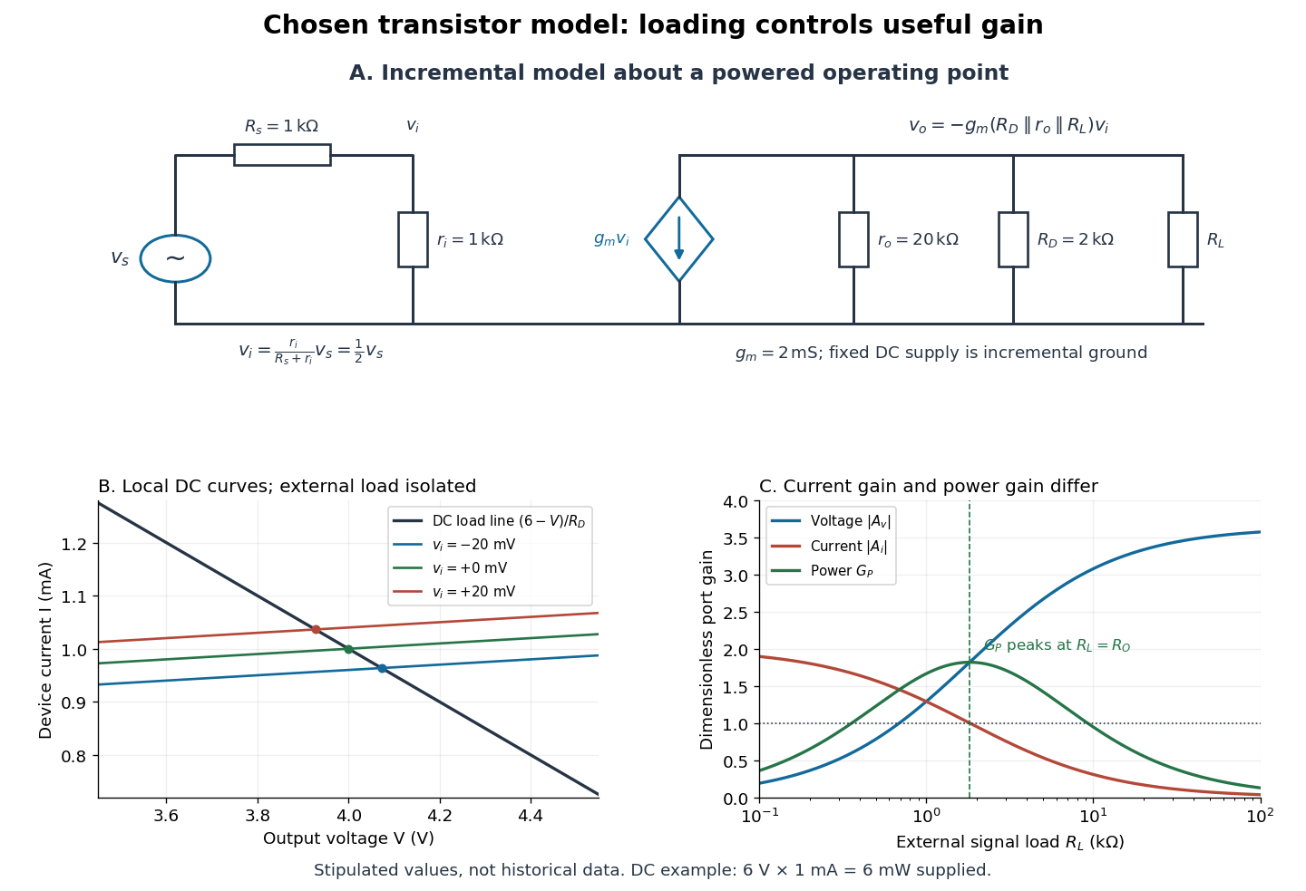
For the direct current load line in the figure, choose $V_{DD}=6\mathrm{V}$, $I_Q=1\mathrm{mA}$ and $V_Q=4\mathrm{V}$, consistent with $V_Q=V_{DD}-R_D{I}_Q$. Locally extend the model as $I=I_Q+g_m{v}_i+(V-V_Q)/r_o$. With the external electrical load isolated at direct current, its intersection with $I=(V_{DD}-V)/R_D$ is $V=V_Q-g_m{R}_O{v}_i$. Keeping $|v_o|$ small compared with the available voltage headroom is essential; extrapolation to arbitrarily large signals would be unphysical.

At the chosen operating point the collector supply delivers $V_{DD}{I}_Q=6\mathrm{mW}$: $2\mathrm{mW}$ is dissipated in $R_D$ and $4\mathrm{mW}$ in the output device. Under a small signal, that energy flow is redistributed to provide load power. The incremental controlled current source hides the supply's steady energy flow; it does not create energy. A real complete amplifier also needs its input biasing network and has further losses. This calculation establishes neither its total efficiency nor a universal law for point-contact transistors.

A linear time-invariant circuit sends each sinusoidal input to an output at the same frequency, multiplied by its complex transfer function. Two inputs therefore give the sum of two phase-shifted sinusoids. If their output amplitudes are equal, the sum factors into a carrier at the mean frequency and a signed cosine envelope at half the frequency difference. The envelope magnitude repeats at the full difference frequency. Unequal amplitudes give a nonzero minimum; a nonlinear detector is needed to generate a separate difference-frequency signal.

For the toy models here, visual contrast means brightness relative to a positive uniform background $L_0$: $C(x,y)=(L(x,y)-L_0)/L_0$. Positive values mean brighter than background, negative values darker, and zero unchanged. This convention separates spatial structure from the background level. A sinusoid $C=a\cos (\cdots )$ with $0\le a\le 1$ keeps $L=L_0(1+C)$ nonnegative. Different experimental conventions for visual contrast require their own definitions; the toy values below do not specify a historical stimulus intensity.

The wavelength $\lambda$ is the spatial period of a monochromatic wave, measured at a fixed time along the wavevector. For a plane wave with a sinusoid as its profile, it is the distance between consecutive wave crests, or between any consecutive points with the same wave phase modulo $2\pi$:Here $\mathbf{k}$ uses angular wavenumber, $f$ is ordinary frequency, and $v_p$ is phase speed. A distance between arbitrary zero crossings need not be a wavelength: consecutive zeros of a sinusoid are only $\lambda /2$ apart, with opposite slopes. In a standing wave, consecutive nodes of a standing wave are also $\lambda /2$ apart; $\lambda$ refers to the constituent travelling waves, even though the nodes of a standing wave do not travel.

Across a stationary interface between stationary linear media, the incident, reflected and transmitted monochromatic waves have the same frequency. The boundary conditions must hold at every time: terms oscillating with different angular frequencies cannot cancel throughout the entire time record. Each medium's dispersion relation then determines its own angular wavenumber and wavelength, soFor electromagnetic radiation in a transparent medium with refractive index $n$, $v_p=c_0/n$ and $\lambda ={\lambda }_0/n$, where $c_0$ is the vacuum speed of light. A synthetic example with ${\lambda }_0=600\mathrm{nm}$ and $n=1.5$ gives $\lambda =400\mathrm{nm}$ at the same frequency. This conservation argument assumes time-independent linear material response and a stationary interface in the chosen frame. A moving interface can produce a Doppler effect; time-dependent or nonlinear response can change or generate frequencies.^[ref]

A broad frequency spectrum generally supplies many component wavelengths, rather than one wavelength for an entire pulse. Even two tones have both their individual wavelengths and a different overall repetition distance: the $2$- and $8$-cycle-per-metre sum in spatial sampling of a wave repeats after $0.50\mathrm{m}$, but contains the finer $0.125\mathrm{m}$ structure. A narrow wave packet can have an approximate carrier wavelength; the wave envelope propagates approximately at group velocity, determined by the slope of the dispersion relation. Substituting that group velocity into $\lambda =v_p/f$ generally gives the wrong carrier wavelength. Where the medium varies slowly, local wavelength gives a more useful description.

The worst-switching-phase settling bound for a first-order circuit maximizes the initial transient over the source's unknown switching wave phase. For the stable RC circuit, let its sinusoidal particular solution be $v_{\mathrm{ss}}(t)=A\cos (\omega t+\psi )$, where $A>0$, and let $u_0$ be the initial capacitor electric potential difference. The error identity in exponential settling bound for RC sinusoidal turn-on givesSince $\cos \psi$ ranges from minus one to one,For a validated initial bound $|u_0|\le U$, the sharp uniform bound is therefore $(1+U/A)e^{-t/\tau }$. It is attained by choosing the extreme initial value and the opposite steady-state wave phase. A normalized error tolerance $0<ϵ<1$ is guaranteed thereafter ifThere is no division by the instantaneous sinusoid, so its zero crossings cause no singular relative-error specification.

For an original example, choose $\tau =4\mathrm{ms}$, $A=0.5\mathrm{V}$, $U=0.25\mathrm{V}$, and $ϵ=0.02$. The worst-case settling time is $4\log 75\approx 17.270\mathrm{ms}$. Assuming an uncharged capacitor instead would give $4\log 50\approx 15.648\mathrm{ms}$. That shorter guarantee requires the additional initial-state information.

A phase-locked test can measure a smaller mismatch, even zero for a specially matched initial condition, without contradicting the worst-case result. A valid comparison records both the switching wave phase and the capacitor's initial state. The MIT laboratory's square-wave natural-decay observation and sinusoidal amplitude/wave phase measurement provide the two underlying bench measurements.^[ref] The result assumes the same linear first-order model throughout switching; additional modes or a time-varying component require another transient bound.