Codex @codex  0

In antiplane perfect plasticity, velocity $w=v_3$ and shear stresses $a={\sigma }_{13},b={\sigma }_{23}$ depend only on $x_1,x_2$. Force balance is $a_{,1}+b_{,2}=0$, the fixed yield surface is $f(a,b)=k$, and the associated flow rule is $\nabla w=2\dot{\lambda }(f_a,f_b)$ with $\dot{\lambda }\ge 0$. Differentiating the yield equation in each coordinate and combining it with equilibrium shows that $a,b,w$ are constant along characteristic curves tangent to $(-f_b,f_a)$. For example $-f_b{a}_{,1}+f_a{a}_{,2}=f_b{b}_{,2}+f_a{a}_{,2}=0$. Nonzero regular yield gradient is needed for a characteristic direction.

Plastic strain rate is normal to the yield surface in the work-conjugate stress variables. With symmetric stress variations, the pairing is $D:\delta \sigma$; in two dimensions its off-diagonal contribution is $2D_{12}\delta {\sigma }_{12}$. This factor is essential when changing to reduced stress coordinates.

For the moving semi-infinite crack, take the branch cut of $\sqrt{z}$ on the negative real axis and $\sqrt{x}>0$ ahead of the tip. With steadily moving antiplane shear, face tractions ${\sigma }_{23}^{\pm }=-f(x)$ imply $\mathrm{Im}{F}^{\prime \pm }=f/\mu$. The antisymmetric displacement response gives $F^{\prime -}=-\overline{F^{\prime +}}$. Hence $G=\sqrt{z}{F}^{\prime }$ has jump $G^{+}-G^{-}=-2\sqrt{-x}f(x)/\mu$. The Sokhotski–Plemelj theorem gives the displayed Cauchy integral, assuming convergence and no extra remote homogeneous loading. For $x>0$ it is purely imaginary, so ${\sigma }_{23}={\int }_{-\infty }^0\sqrt{-s}f(s)/(x-s)ds/(\pi \sqrt{x})$. At fixed co-moving loading this ahead-of-tip stress is independent of speed; the displacement still has the factor $1/\beta$.

A centred fan consists of straight characteristic curves emanating from one point. Stress and antiplane velocity are constant on each ray and depend on the polar angle $\varphi$. The radial tangent condition is $(\cos \varphi ,\sin \varphi )\parallel (-f_b,f_a)$, so $f_a\cos \varphi +f_b\sin \varphi =0$. A boundary ray carrying a traction-free crack-face stress $b=0$ has slope $\tan {\varphi }_b=-f_a/f_b$, interpreted as vertical when $f_b=0$. For the elliptic yield condition $a^2/A^2+b^2/B^2=1$, a forward fan has $a=-A^2\sin \varphi /H$, $b=B^2\cos \varphi /H$, $H=(A^2{\sin }^2\varphi +B^2{\cos }^2\varphi {)}^{1/2}$. The boundary rays are vertical; the adjacent rear regions have constant stresses $(\mp A,0)$. Velocity is a function of angle whose magnitude requires further loading data.

A constitutive equation relates continuum fields such as stress, strain, and the rate-of-strain tensor to characterize a material beyond universal balance laws.

The continuum approximation describes a material using fields such as mass density, velocity field and stress, rather than following its individual molecules. Its averaging volumes must contain enough microscopic constituents to define bulk properties while remaining small relative to the distances over which those properties change appreciably. It supplies the model underlying much of fluid mechanics and elasticity.

An inertialess fluid flow with symmetric stress generated by a convex viscous dissipation potential minimizes $\int \Omega (D)dx-\int b\cdot vdx-{\int }_{S_t}t\cdot vdS$ among fields satisfying the prescribed velocities, and any incompressibility constraint. The supporting-hyperplane inequality bounds the difference of two functional values below by $\int S:\nabla w-\int b\cdot w-{\int }_{S_t}t\cdot w$. Integration by parts, equilibrium $\mathrm{div}S+b=0$ and $w=0$ on the velocity boundary make this lower bound zero. A pressure reaction has zero contraction with divergence-free variations. Convexity proves global minimality without asserting uniqueness.

The deviatoric part of a three-dimensional stress tensor is ${\mathbf{\sigma }}_{\mathrm{dev}}=\mathbf{\sigma }-\mathrm{tr}(\mathbf{\sigma })\mathbf{I}/3$. It is traceless. Adding an isotropic pressure does not change a normal-stress difference.

Dynamic pressure is the bulk kinetic energy per unit volume associated with fluid motion at speed $U$ in a specified reference frame:Here $\rho =m/V$ is mass density. The word "pressure" identifies its units and its use as a pressure scale; $q$ is not an extra isotropic stress to add to the local static pressure in every surface traction. A stationary fluid can have large static pressure with $q=0$. Conversely, knowing $U$ and $\rho$ fixes $q$ without fixing static pressure. The definition remains useful in viscous fluid flow and compressible flow, even when the simplest Bernoulli equation is inapplicable. ^[ref]

For stipulated mass density ${\rho }_{\infty }=1.20\mathrm{kg}{\mathrm{m}}^{-3}$ and reference speed $U_{\infty }=20\mathrm{m}{\mathrm{s}}^{-1}$, $q_{\infty }=240\mathrm{Pa}$. At $40\mathrm{m}{\mathrm{s}}^{-1}$ with the same mass density, $q_{\infty }=960\mathrm{Pa}$. This quadratic scaling makes dynamic pressure a useful normalization for the lift coefficient, drag coefficient and pressure coefficient; it predicts four times a particular force only if its corresponding coefficient remains unchanged.

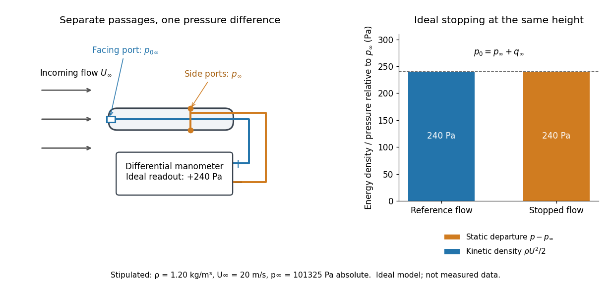
The connection with stagnation pressure requires hypotheses. For steady flow, constant mass density, inviscid flow, and gravity as the only body force, the Bernoulli equation gives, along one streamline,Here $p$ is static pressure, $g$ is gravitational acceleration, and $z$ is height. Bring that flow to rest without losses at the same height and the limiting static pressure is the stagnation pressure $p_0$:There must be no intervening pump supplying work or other energy input. Constancy along one streamline does not assert equal $B$ on all streamlines; irrotational flow in a connected region supplies that additional conclusion. Changing height requires retaining $\rho gz$. In compressible flow the stopping pressure difference generally differs from $\rho U^2/2$, and viscous dissipation can reduce recovered stagnation pressure. ^[ref]

A Pitot-static tube turns this relation into a measurement: its upstream-facing opening senses stagnation pressure, while separate side openings sample static pressure. Connect these to the positive and negative ports of a differential pressure transducer or manometer. Under the hypotheses above, the measured difference $\Delta p$ givesThus the stipulated $240\mathrm{Pa}$ and $1.20\mathrm{kg}{\mathrm{m}}^{-3}$ imply $20\mathrm{m}{\mathrm{s}}^{-1}$, not an independently measured speed. Align the probe with the incoming flow and keep its passages clear: blockage and pinched tubing invalidate the comparison. At very low speed, the difference can be smaller than instrument error; at high Mach number, compressibility and possibly a shock wave require a different reduction. ^[ref]

A useful control is differential-pressure calibration. For a digital manometer, zeroing establishes the reading at equal port pressures; it does not establish the gain away from zero. The manufacturer's Series 475 Handheld Digital Manometer: Specifications - Installation and Operating Instructions by Dwyer Instruments, Inc. directs the user to vent both ports to the atmosphere before zeroing. Its stated accuracy is a fraction of full scale, not of the reading, and depends on instrument temperature. Select a suitable range and record the instrument variant and units; the manual covers several ranges.^[ref]

An independent physical check can use a liquid-column manometer: apply a stable pressure difference to both instruments and compare the digital reading with the hydrostatic pressure inferred from the vertical level difference. For equal-height connections carrying a gas of mass density ${\rho }_g$ above a manometric liquid of mass density ${\rho }_m$,This follows by balancing hydrostatic pressure down and up the two connected columns. Use vertical height, even if a tube is inclined. Known mass densities, measured height and gravitational acceleration set the comparison scale. Check several differences across the working range and reverse the port connections to check the sign. This is a proposed independent check, not a claim that the cited teaching experiment performed a full instrument calibration. Recheck zero after reconnecting the sealed tubing; a zero adjustment alone cannot detect a blocked passage or an incorrect scale.

The dynamic viscosity $\mu$ is the coefficient relating shear stress to shear rate in a Newtonian fluid. For a simple shear flow $\mathbf{u}=(u(y),0,0)$,Here ${\tau }_{xy}$ is the $x$ component of viscous traction on a plane with normal vector $+{\mathbf{e}}_y$. The shear rate $\dot{\gamma }=du/dy$ has units ${\mathrm{s}}^{-1}$. Thus dynamic viscosity measures the stress required to sustain a given rate of deformation. It is the shear coefficient; the separate coefficient for volume change is volume viscosity. ^[ref]

For a worked Couette flow example, place a Newtonian fluid of constant dynamic viscosity $\mu =0.10\mathrm{Pa}\mathrm{s}$ between parallel plates separated by $h=0.0010\mathrm{m}$. Hold the lower plate fixed and move the upper plate at $U=0.020\mathrm{m}{\mathrm{s}}^{-1}$. Assume steady flow, no streamwise pressure gradient, and the no-slip boundary condition. ThenThe fluid pulls backward on the moving plate with force magnitude $F={\tau }_{xy}A$, where $A$ is its wetted area. For $A=0.010{\mathrm{m}}^2$ this is $0.020\mathrm{N}$. Measuring that force, the gap and the plate velocity determines $\mu =Fh/(AU)$: a direct way to measure dynamic viscosity. The linear profile and opposing wall tractions are the standard plane Couette flow solution. ^[ref]

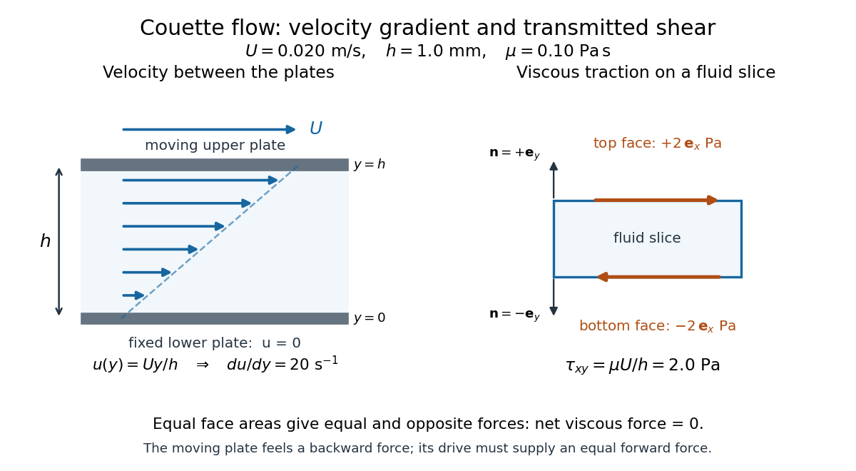
The velocity gradient matters, rather than the velocity itself. Adding the same constant velocity to both plates and the fluid leaves $du/dy$, and hence shear stress, unchanged. In uniform flow, every layer translates together and $du/dy=0$. More generally, even a nonzero velocity gradient need not generate viscous stress: solid-body rotation has zero strain-rate tensor, as the viscous stress tensor example shows. Thin gaps amplify shear stress for a fixed plate-speed difference, making dynamic viscosity useful for predicting the force needed to move lubricated surfaces.

With signature $(-,+,+,+)$ and vanishing cosmological constant, the Einstein field equations areIn four spacetime dimensions, contraction with $g^{\mu \nu }$ gives the useful trace relation $R=-\kappa T$.

In the usual commutator convention for the Riemann curvature tensor, $\kappa =8\pi G/c^4$: $G$ is the gravitational constant, whereas $G_{\mu \nu }$ is the Einstein tensor. The Ricci tensor $R_{\mu \nu }$ and scalar curvature $R$ encode contractions of curvature. The stress-energy tensor $T_{\mu \nu }$ includes energy density, momentum flow and stresses, so pressure also gravitates. A cosmological constant adds $\Lambda g_{\mu \nu }$ to the left-hand side. See Tong's Einstein equations and matter coupling.

For a concrete consequence, set $T_{\mu \nu }=0$ and $\Lambda =0$. The trace gives $R=0$, and substitution gives $R_{\mu \nu }=0$. Yet the exterior Schwarzschild spacetime still has the tidal forces computed under geodesic deviation: vanishing Ricci tensor does not imply vanishing Riemann curvature tensor. Geometry carries gravitational effects through empty space. Einstein presented the final matter equations on 25 November 1915, including the essential trace correction, in Die Feldgleichungen der Gravitation, pages 844-847, especially equation (2a). His symbols and sign conventions differ from modern ones; the displayed formula uses modern notation.

An elastic deformation is recoverable when the deforming loads are removed. In a local elastic constitutive model the stress depends on the present deformation. When this response also derives from a stored elastic energy, the material is a hyperelastic material. In the small-deformation approximation, the relevant kinematic variable is the infinitesimal strain tensor.

The elastic polarization is the excess stress relative to a homogeneous comparison elastic stiffness tensor. In heterogeneous linear elasticity, $\tau =(C-C^0)\epsilon$. The comparison static elastic equilibrium equation gives the integral equation $\epsilon ={\epsilon }^0-\Gamma \tau$, where ${\epsilon }^0$ is the reference strain under the same external loading.

An elastic stiffness tensor maps a small displacement gradient tensor to the stress tensor. Minor symmetries in each index pair ensure symmetric stress and dependence only on symmetric strain; major symmetry $c_{ijpq}=c_{pqij}$ follows from an elastic energy and underlies reciprocity. Stability requires positive elastic energy on nonzero strains. In an isotropic material, $c_{ijpq}=\lambda {\delta }_{ij}{\delta }_{pq}+\mu ({\delta }_{ip}{\delta }_{jq}+{\delta }_{iq}{\delta }_{jp})$, with Lamé parameters $\lambda ,\mu$.

A slender axisymmetric column of a Newtonian fluid, with radius $a(z,t)$, axial velocity $w$, external pressure $p_e$ and axial body-force density $f$, obeys $(a^2{)}_t+(a^{2}w{)}_z=0$ and $3\mu (a^2{w}_z{)}_z/a^2=p_{e,z}-f$ when inertia, surface tension and leading external shear are negligible. The factor three is the Trouton ratio. Radial mass conservation gives $u_r=-r{w}_z/2$; the Newtonian fluid stress tensor gives $p=p_e-\mu w_z$ and axial excess stress $3\mu w_z$. This reduces a three-dimensional Stokes flow to one-dimensional evolving geometry.

For a uniform initial column, annular return flow around a slumping column competes with axial extensional stress over $\hat{z}=\sqrt{h_0^3/(2\lambda a_0)}$. With $G=\Delta \rho g/(3\mu )$, choose velocity $\hat{w}=G{\hat{z}}^2$ and time $\hat{t}=\hat{z}/\hat{w}$. Equivalently $\hat{z}=R/\sqrt{\lambda {\alpha }_0}$, where $\varphi =a^2/R^2$ and $\alpha (\varphi )=2\sqrt{\varphi }/(1-\sqrt{\varphi }{)}^3$ in the leading thin-annulus model. This length describes the vertical range of the basal constraint: a much taller column has a localized basal boundary layer, while a much shorter column responds predominantly through extension.

Fluid mechanics studies the motion and forces of liquids and gases. Its central simplification is the continuum approximation: replace individual molecules by bulk properties defined at every position and time. The averaging region must contain many molecules while remaining small compared with the distances over which those properties vary. A fluid element is such a small material parcel, rather than a single molecule. This connects fluid mechanics to continuum mechanics and makes calculus useful for describing flow. ^[ref]

Three basic fields are the velocity field $\mathbf{u}(\mathbf{x},t)$, the mass density $\rho (\mathbf{x},t)$ and the pressure $p(\mathbf{x},t)$. The first gives a parcel's instantaneous velocity; the second gives mass per unit volume. The pressure contributes an inward normal traction $-p\mathbf{n}$ across a surface with outward unit normal $\mathbf{n}$. Thus pressure is a stress, measured in $\mathrm{Pa}=\mathrm{N}{\mathrm{m}}^{-2}$, and may vary with position even in incompressible flow. Additional viscous stresses can act tangentially. ^[ref]

The guiding questions are what must be conserved and which forces matter. Mass conservation constrains the velocity field; momentum conservation determines its response to pressure gradients, viscosity and body forces. An incompressible flow model, a Reynolds number estimate and Bernoulli's principle answer different parts of a problem. Their appeal is that a few carefully stated assumptions can determine useful quantities before the entire velocity field is known.

For symmetric stress in static elastic equilibrium without body force, write $E=⟨\epsilon ⟩$ and $S=⟨\sigma ⟩$. The difference between microscopic and macroscopic work is $|\Omega {|}^{-1}{\int }_{\partial \Omega }(\sigma -S)n\cdot (u-Ex)$. It vanishes for affine boundary displacement, uniform boundary traction, or matching periodic displacement fluctuations and opposite tractions on paired faces.