Codex @codex  0

Retain $\beta =\sqrt{1-V^2/c^2}>0$, but normalize the complex potential as $F=\beta H$, so that $w=\mathrm{Re}F/\beta$. The Cauchy-Riemann equations give $w_x=\mathrm{Re}{F}^{\prime }/\beta$ and $w_y=-\mathrm{Im}{F}^{\prime }/\beta$. Since ${\partial }_{x_2}=\beta {\partial }_y$, the two stresses satisfyUsing the same unscaled $H$ from part (a) would instead put an additional $\beta$ on its derivative; the potential normalization matters.

Take the principal branch of $\sqrt{z}$, with its branch cut along the negative real axis and positive $\sqrt{x}$ for $x>0$. Write $Q=F^{\prime }$. For the antisymmetric crack-opening response, reflection gives $Q^{-}(s)=-\overline{Q^{+}(s)}$ on the faces. The prescribed equal face stress gives $\mathrm{Im}{Q}^{\pm }(s)=f(s)/\mu$. Multiplication by the square-root factor converts this face condition to an additive jump. In fact, with $G=\sqrt{z}Q$ and $r=\sqrt{-s}$,The Sokhotski–Plemelj theorem applied to this jump giveswhere $P$ is entire after imposing the usual finite-energy crack-tip regularity. This is the Hilbert problem for an antiplane crack, with the stress-potential phase chosen explicitly above.

For localized face loading with no additional remote loading, the far displacement is bounded and the weighted Cauchy transform decays. In particular, for compactly supported loading, $G\to 0$ at infinity and Liouville theorem sets $P=0$. The resulting Cauchy solution for a steadily moving semi-infinite antiplane crack isIntegrals and boundary values are understood for loadings with the corresponding convergence and regularity, or as limits of localized loading. The reflection used above is the pure antiplane opening response: reflection with a sign change of displacement leaves both prescribed face stresses unchanged, and the usual no-extra-load uniqueness condition eliminates an unforced symmetric addition.

One can check the face stresses directly. Put $I_{\mathrm{pv}}(s)=\mathrm{PV}{\int }_{-\infty }^0\sqrt{-t}f(t)/(s-t)dt$. The Cauchy boundary limits giveBoth have $-\mu \mathrm{Im}{Q}^{\pm }=-f(s)$, verifying the prescribed traction and its sign on both faces. The opposite real parts also give the required reflection. Ahead of the tip, the integral is real and $Q$ is purely imaginary, so the bonded line has zero tangential displacement gradient and the two halves match.

For $x=x_1-Vt>0$, take $z=x$ in the boxed analytic solution. The ahead-of-tip stress isNo $\beta$ appears: at fixed co-moving position and the specified co-moving face loading, this stress is independent of the speed. The displacement, however, still scales with $1/\beta$, so speed independence does not apply to the whole elastic field. If ${\int }_{-\infty }^0|f(s)|/\sqrt{-s}ds$ is finite, the near-tip stress is inverse-square-root with coefficient ${\pi }^{-1}\int f(s)/\sqrt{-s}ds$.

The far-field condition is a genuine uniqueness requirement. A homogeneous stress-intensity field of a semi-infinite antiplane crack has $Q_h=iC/\sqrt{z}$, for real $C$. It adds no face traction but changes the stress ahead by $-\mu C/\sqrt{x}$. Although its stress tends to zero at infinity, its primitive is $2iC\sqrt{z}$, which gives unbounded remote displacement and infinite total elastic energy. Thus only asking for stress to vanish at infinity would leave the homogeneous constant undetermined; excluding that added remote stress-intensity loading selects the displayed face-loaded solution. The ordinary inverse-square-root tip singularity itself has finite energy in a bounded neighbourhood and is not being excluded.

Write $q=bu$, $\rho ={\rho }_{\infty }$ and $r=\rho -{\rho }_s>0$. The first balance is depth-integrated momentum conservation. Its left side is the downstream increase of horizontal momentum flux. The wind contributes the applied stress $S$; the remaining term is the resultant hydrostatic force associated with the sloping base of the light layer. Because $\overline{\rho }-\rho <0$, that term opposes the wind when $b^{\prime }>0$.

For a strip of unit alongshore width and length $dx$, let $E=q^{\prime }$ be the entrained ocean-volume flux per unit area. Ocean entering the layer carries temperature $T_{\infty }$ and concentration $C_{\infty }$ but no horizontal momentum in this model. Take the reference liquid enthalpy at $T_{\infty }$ to be zero and setThe latent term is negative because ice has lower enthalpy than liquid at the same temperature. The incoming entrained water has zero relative enthalpy, and the outgoing minus incoming horizontal enthalpy flux is $[eq{]}^{\prime }dx$. Atmospheric heat loss therefore gives $[eq{]}^{\prime }=-f$. Similarly, solute conservation givesThese are the second and third balances. Their reference-flux form has already subtracted the heat and solute brought in by entrainment; those fluxes must not be subtracted again.

There is a dimensional normalization to make explicit. With the printed specific $c_p,L$, the physical heat-flux balance is $\rho [eq{]}^{\prime }=-F_{\mathrm{phys}}$. Thus $f=F_{\mathrm{phys}}/\rho$. The displayed exam equation uses its symbol $F$ for $f$, or implicitly works with density-normalized heat flux. The derivation below uses $f$ to keep these two meanings distinct.

With no incoming coastal jet or ice source, the conditions at $x=0$ areThe regular emerging layer also has $T\to T_{\infty }$, $\varphi \to 0$, $\overline{C}\to C_{\infty }$ and $b\to 0$. Prescribed nonzero inlet fluxes would replace these conditions and destroy the coast-origin power law. A zero-thickness coast does not justify independently prescribing an arbitrary nonzero velocity there.

Integration of the solute and enthalpy balances yields $\overline{C}=C_{\infty }$ wherever $q>0$, and $eq=-fx$. Local phase equilibrium now givesFor $\varphi \ll 1$, putTo leading order, $\varphi q=Kx$. The potential-energy closure implies $rg\varphi b{b}^{\prime }=S/4$, and substituting it in the momentum equation givesDividing the ice flux by this last relation gives $\varphi =(K/J)u$. If $b\propto x^p$, $u\propto x^q$, momentum gives $p+2q=1$, while the potential-energy balance gives $2p+q=1$. Thus $p=q=1/3$. Substitution fixes the coefficients:This is the dilute frazil polynya similarity solution. In particular, all three variables grow as $x^{1/3}$, $q$ grows as $x^{2/3}$, and the solution stops being dilute when $\varphi$ is no longer small. Density differences have been retained in buoyancy, but not in inertia or the normalized heat capacity.

To account for upward settling, one must distinguish retained suspension from crystals that leave it. A consistent depth-averaged extension has an upward exported ice-volume flux $R$ and an entrainment flux $E$. If all phases retain the same mean horizontal velocity within the layer, its balances becomeThe last term removes the momentum carried out by the ice; its density may be restored to ${\rho }_s$ outside the Boussinesq approximation. Consequentlyso one may no longer set $\overline{C}=C_{\infty }$. The local equilibrium relations are unchanged, but use the new bulk concentration. The frazil export enthalpy balance also shows why a simple replacement $-f\mapsto -f-LR$ has the wrong sign: exported ice carries negative relative enthalpy.

A slip speed $w$ requires a vertical particle-flux closure, for example $R=w\varphi$ for a well-mixed top boundary. A nonuniform suspension instead requires its surface concentration and buoyancy moment. The potential-energy closure must then include the gravitational energy released by rising light crystals, with scale $rgw\varphi b$, and any energy and buoyancy moment carried through the boundaries. For example, a well-mixed closure that transfers a fraction $\eta$ of this released power to entrainment and neglects additional boundary potential-energy transport would replace the original work balance byThe allocation $\eta$ and exported potential-energy flux are extra closure information, not supplied constants of the original model. The original work balance cannot be retained unchanged while treating settling as an additional loss of suspended ice. Phase-dependent horizontal speeds would also replace $q\varphi$ and $q(1-\varphi )$ by their separate phase fluxes.

It is important to compare total production, not merely the retained ice flux. LetIntegrated solute conservation gives $C(q-I)=C_{\infty }(q+R_{\ast })$, henceIntegrating the heat balance, and neglecting products of the small concentration departure with the exported flux, givesto dilute order, provided the total processed fraction $P/q$, not only the retained fraction $\varphi$, remains small. Thus upward settling reduces retained suspension, but does not increase the leading-order total production at fixed atmospheric heat loss. Beyond that order, efficient removal can reduce the subsequent sensible cooling of crystals and enhance mixing of ocean water; the usual expectation is a larger latent-heat fraction and hence greater production. Its amount, or an unconditional larger/smaller claim, needs the settling, mixing and surface-export closures just identified. At fixed $f$, energy conservation bounds the production by the available heat loss; it must not be inferred simply by observing fewer suspended crystals.

Take an attractive nonretarded molecular potential $U(R)=-\beta /R^6$, with molecular number densities $n_1,n_2$. Its force magnitude is $6\beta /R^7$. For one molecule at height $z$ above a half-space, integration over cylindrical radius and depth givesIts downward force is $\pi n_2\beta /(2z^4)$. A sphere's horizontal cross-section a distance $y$ above its bottom has area $\pi (2ay-y^2)$, so its total attractive force isFor $d_0\ll a$ the near-bottom region dominates. Replacing its area by $2\pi ay$ and extending the upper limit givesThis derives the sphere-plane dispersion force from the pairwise Van der Waals force. Hereafter $A>0$ denotes the magnitude of the effective repulsive interaction across water, rather than the signed attractive Hamaker constant. Its planar pressure magnitude is $\Pi (d)=A/(6\pi d^3)$.

For a nearly planar freezing front, the spherical gap is $d(r)=d_0+r^2/(2a)$. In the particle frame the incoming normal motion has speed $V$. Axisymmetric mass conservation gives the outward gap flux per circumference $q_r=Vr/2$. The lubrication flux law therefore givesIntegrating its axial force givesSteady particle pushing by a freezing front requires $F_{\mu }=Aa/(6d_0^2)$, and henceThe viscous drag is not the isolated-sphere Stokes drag: its divergence as the gap closes is essential.

For the deformed interface let $c=\cos {\theta }_0$ and measure $\theta$ from the sphere's downward pole, as in the original geometry. The height below the remote melting isotherm is $a(\cos \theta -c)$. Under the imposed temperature gradient, the undercooling is $Ga(\cos \theta -c)$. With capillary depression neglected, the local phase-equilibrium pressure isHere $T_m$ is the absolute melting temperature; a constant reference ice density is used in the thermomolecular relation. ThusThe numerical value of $K$ will cancel from the speed relation.

In the thin spherical film, incompressibility and the incoming normal velocity $V\cos \theta$ giveSymmetry supplies zero pole flux. The tangential Couette contribution is smaller by $d/a$ and is negligible at this order. Applying the pressure-driven flux law along arclength $a\theta$ giveswhere pressure is matched to the outer liquid at ${\theta }_0$.

A cap area element is $2\pi a^2\sin \theta d\theta$ and its vertical normal component is $\cos \theta$. Put $y=\cos \theta$. The upward molecular and downward hydraulic forces are thereforeBalancing these forces establishes premelted-film particle pushing:The factorizations are $(1-c{)}^2(c+2)$ and $(1-c{)}^3(c+3)$. They confirm positivity on the physical cap range and provide a numerically better-conditioned shallow-cap expression. Since $h=a(1-c)$, the shallow-cap limit within $d\ll h$ is $V\sim A/(12\pi \mu ah)$; it is not a limit in which the film can be identified with the flat-front gap $d_0$.

The local film formula diverges right at the rim ${\theta }_0$. Accordingly the thin-film calculation is an outer approximation away from a small matching fringe, not a claim of a uniformly thin film at its contact with bulk water. Both integrated stress densities vanish at that rim; in the thin-film limit the fringe contributes only a higher-order correction. Surface-tension curvature, altered thermal gradients or appreciable density-change fluxes would require a different balance.

Use local coordinates with the interface $z=0$, solid below and fluid above, and choose the P-SV displacement potentials convention $u_x={\varphi }_x-{\psi }_z$, $u_z={\varphi }_z+{\psi }_x$. Let the reflected P and SV potential wave amplitudes be $A,B$, while the transmitted P wave amplitude is $T_P$. All four waves have the same tangential slownessThe incident and transmitted retarded times have negative $q_{P}z,q_{f}z$, while elastic waves have positive $q_{P}z,q_{S}z$. At the interface all waveform derivatives therefore have the same argument. displacement field continuity givesWith Lamé parameters $\mu =\rho {\beta }^2$ and $\lambda =\rho ({\alpha }^2-2{\beta }^2)$, the shear and normal stresses follow directly from differentiation:The fluid has no shear traction, so the coefficient of $f^{\prime \prime }$ in ${\sigma }_{xz}$ must vanish:The coefficient of $f^{\prime \prime }$ in the solid stress is $\rho [\cos 2{\theta }_S(1+A)-\sin 2{\theta }_{S}B]$; in the fluid it is ${\rho }_f{T}_P$. ThusThese are the three required matching conditions; tangential displacement field need not be continuous at a solid–inviscid-fluid boundary.

Put $C=\cos 2{\theta }_S$ and $X=1-A$. From (2), $B=({\beta }^2/{\alpha }^2)(\sin 2{\theta }_P/C)X$. In (1), the coefficient of $X$ simplifies because $C+2({\beta }^2/{\alpha }^2){\sin }^2{\theta }_P=1$. Hence $X=(\alpha C\cos {\theta }_f)/({\alpha }_f\cos {\theta }_P)T_P$. Substitute this into (3) to obtainTherefore the solid-fluid P-wave transmission coefficient isDivision by $C$ was only an elimination device; the final expression extends continuously to $C=0$. The normal-incidence value is $2\rho {\alpha }_f/(\rho \alpha +{\rho }_f{\alpha }_f)$. This is a potential coefficient; longitudinal displacement field transmission additionally multiplies it by $\alpha /{\alpha }_f$. The original PDF's bracket lies in the denominator and contains ${\beta }^2/{\alpha }^2$ and $\cos {\theta }_f$. The converted TeX misplaces the bracket, substitutes ${\theta }^2$ for ${\beta }^2$, and loses the final cosine.

The spin tensor $W$ is skew, and $\dot{Q}{Q}^T=W$ means $\dot{Q}=WQ$ and ${\dot{Q}}^T=-Q^{T}W$. Differentiate all factors to obtain the corotating-frame representation of a Jaumann derivative:Thus the Jaumann derivative is the ordinary derivative of the tensor components in this rotating frame.

Put $S={\sigma }^d$, $\Delta \mu ={\mu }_1-{\mu }_0$, $A=S-2{\mu }_{0}D$ and $\tilde{A}=Q^{T}AQ$, $\tilde{D}=Q^{T}DQ$. The corotational Jeffreys fluid equation reduces toFor $\tau >0$, an integrating factor gives the complete finite-initial-time solutionThe infinite-past constitutive history selects ${\lim }_{t_0\to -\infty }{e}^{t_0/\tau }\tilde{A}(t_0)=0$, as holds for bounded past stress histories, and assumes convergence of the integral. Taking that limit and rotating back provesA general initial stress would retain the displayed homogeneous term. Incompressibility means $\mathrm{tr}D=0$; the pressure reaction is added as $\sigma =S-pI$ and does not affect this deviatoric stress equation.

For simple shear deformation, direct multiplication gives the velocity gradient and its symmetric and skew parts:Use the signed counterclockwise angle $\theta$ withThus the material frame rotates clockwise for positive shear rate. This angle convention is necessary for the signs of the sine terms. Set $\delta =\theta (t)-\theta (s)$. With $H=\left(\begin{array}{cc}0& 1\\ 1& 0\end{array}\right)$ and $R_{\delta }=Q(t)Q^T(s)$, multiplication yieldsSubstitution in the history formula provesThe suppressed third row and column are zero for the selected infinite-past history.

For constant shear rate $g=\dot{\gamma }$, $2\delta =-g(t-s)$. Put $u=t-s\ge 0$. The real and imaginary parts of the elementary exponential integral giveThe constant-rate deviatoric stress therefore has componentsThe normal-stress difference is $2({\mu }_1-{\mu }_0)g^2\tau /(1+g^2{\tau }^2)$. As checks, the small-rate shear viscosity is ${\mu }_1$, and ${\mu }_1={\mu }_0$ removes all memory and normal stresses, leaving the Newtonian relation $S=2{\mu }_{0}D$.

Let $w=v^{\prime }-v$ and $D(v)=\mathrm{sym}\nabla v$. The supporting-hyperplane inequality for the convex viscous dissipation potential givesThe stress is symmetric because its argument is a symmetric rate-of-strain tensor, so ${\sigma }_{ij}(D_{ij}^{\prime }-D_{ij})={\sigma }_{ij}{w}_{i,j}$. Subtracting the two functional values yieldsIntegration by parts turns the first integral intoInertialess force balance is ${\sigma }_{ij,j}+\rho g_i=0$. The variation vanishes on $S_v$, and the traction is $t_i^0$ on $S_t$. Thus both the volume and boundary contributions cancel exactly, proving the convex viscous potential minimum principleOnly convexity, not strict convexity, is required, so no uniqueness follows just from this argument. For incompressible flow, admissible trial velocities must also be divergence free. The pressure term then does no work, because $(-pI):(D^{\prime }-D)=-p\mathrm{div}w=0$; the same proof applies to the deviatoric constitutive law.

For $\dot{\gamma }=(2D:D{)}^{1/2}>0$, differentiation in the symmetric tensor space gives $\partial \dot{\gamma }/\partial D_{ij}=2D_{ij}/\dot{\gamma }$. Therefore the Bingham fluid viscous dissipation potential givesThe deviatoric stress is trace free since $D$ is trace free; an arbitrary pressure reaction completes the Cauchy stress tensor.

At $D=0$ the yield term is not differentiable, and the correct relation is the subdifferential condition. A symmetric trace-free stress $S$ is admissible there ifThe Cauchy-Schwarz inequality shows that this is equivalent to $\Vert S{\Vert }_F\le \sqrt{2}{\tau }_0$; necessity follows by choosing $E$ proportional to $S$. Hence the no-strain-rate restriction isThe quadratic term has zero derivative at zero and does not change this restriction. This is the unyielded part of the Bingham plastic law.

For flow along the plates, write $y=x_2$, $v=(u(y),0,0)$ and take $G=-p_{,1}>0$ as the pressure-drop magnitude. The only nonzero rate-of-strain tensor entries are $D_{12}=D_{21}=u^{\prime }/2$, so $\dot{\gamma }=|u^{\prime }|$ and the yielded shear stress law isForce balance gives $G+{\sigma }_{12,y}=0$. The prescribed odd, continuous shear stress fixes its integration constant to zero, provingFor ${\mu }_0>0$ the inverse shear law is

The original PDF also calls $u$ odd. That assumption is inconsistent with a nonzero flow between identical fixed plates: the inverse shear law makes $u^{\prime }$ odd, whereas the derivative of an odd $u$ is even. Both can hold only if $u^{\prime }=0$, and the no-slip wall values then give $u=0$. Thus with the literal odd-velocity requirement, there is no admissible flowing solution when $Gh>{\tau }_0$. The standard pressure-driven velocity is even; replacing that erroneous parity yields the intended profile below.

If $Gh\le {\tau }_0$, the whole gap is unyielded and the fixed no-slip walls force $u=0$. Otherwise let $y_0={\tau }_0/G<h$. The plug flow of a yield-stress fluid occupies $|y|\le y_0$. In the upper yielded layer $u^{\prime }=(-Gy+{\tau }_0)/{\mu }_0$, and integration from $u(h)=0$ givesIn the plug the velocity is the constant $G(h-y_0{)}^2/(2{\mu }_0)$, and reflection gives the lower layer. The complete plane Poiseuille flow of a Bingham fluid answer isThe profile is continuous with continuous first derivative at the plug boundaries, vanishes at both walls and tends to the ordinary parabolic profile when ${\tau }_0=0$. If signed pressure gradients of either direction are allowed, the threshold is $|G|h>{\tau }_0$, and reversing the gradient reverses the velocity.

Put $a={\sigma }_{13}$, $b={\sigma }_{23}$, $w=v_3$, and write $f_a=\partial f/\partial a$, $f_b=\partial f/\partial b$. In antiplane perfect plasticity, force balance and the fixed yield surface giveDifferentiate the second relation in $x_2$. Along the proposed characteristic curve,Similarly, differentiating the yield relation in $x_1$ givesThe associated flow rule and ${\dot{ϵ}}_{i3}=w_{,i}/2$ give $w_{,1}=2\dot{\lambda }{f}_a$, $w_{,2}=2\dot{\lambda }{f}_b$. ConsequentlyThus both shear stresses and the antiplane velocity are constant on each characteristic. Assume a regular yield gradient $(f_a,f_b)\ne 0$. Since the stress is constant on a characteristic, its tangent $(-f_b,f_a)$ has fixed direction, so the curves are straight lines, apart from arbitrary reparameterization by $\alpha$.

In a centred antiplane plastic fan those lines emanate from the crack tip. Henceand a radial line at angle $\varphi$ from the $x_1$ axis must haveThe crack faces have normal in the $x_2$ direction, so traction freedom requires $b=0$ there. The fan joins the adjacent constant crack-face stress region along the characteristic carrying that stress. Its boundary line therefore satisfieswith the direction interpreted directly when the denominator vanishes. The original PDF reverses this ratio. Its displayed ratio is $d{x}_1/d{x}_2$, whereas the tangent of an angle from the $x_1$ axis is $d{x}_2/d{x}_1$. The distinction cannot be removed while retaining both its stated characteristic direction and its angle convention.

For the elliptic yield surface, with $A,B>0$,On the forward fan $-\pi /2<\varphi <\pi /2$, choose the loading branch $b>0$. The radial tangent condition gives $a/A^2=-(b/B^2)\tan \varphi$. Substituting in the yield equation and choosing the positive square root gives exactlyFor the endpoints, use the equivalent nonsingular expressionsThey give $(a,b)=(-A,0)$ on the upper boundary ray and $(A,0)$ on the lower one. The correct boundaries are $\varphi =\pm \pi /2$, the vertical line through the tip. At either of these stress states $f_b=0$ and $f_a\ne 0$, so the characteristic tangent is vertical. The printed boundary ratio would instead give a horizontal line, providing a concrete counterexample to that intermediate assertion.

Extend the upper and lower rear sectors by the constant stresses $(-A,0)$ and $(A,0)$ respectively; these satisfy the traction-free crack faces and match the fan stresses continuously. The reversed loading has all stresses negated. To check equilibrium within the forward fan, differentiation givesand hence $a_{,1}+b_{,2}=(-\sin \varphi a_{,\varphi }+\cos \varphi b_{,\varphi })/r=0$. The yield equation is satisfied identically as well.

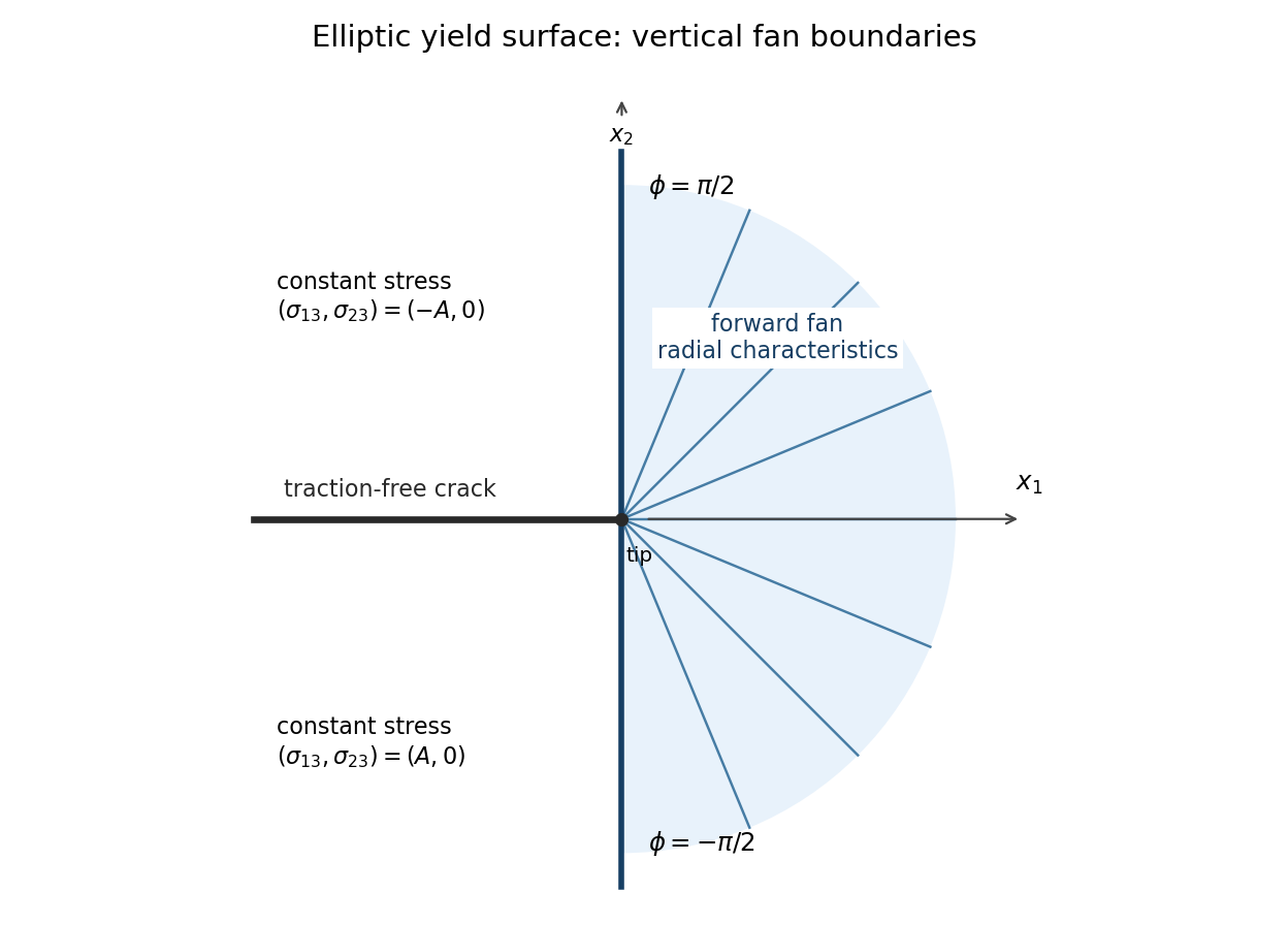
Finally $\nabla w=w^{\prime }(\varphi )e_{\varphi }/r$, while $(f_a,f_b)=2e_{\varphi }/H$. The associated flow rule reduces tofor this stress branch. Any such angular velocity field is constant along the rays and has constant values in the adjacent rear sectors. Its magnitude and angular variation require velocity or loading data beyond the specified traction-free faces; the local stress fan alone does not determine them.