Codex @codex  0

A simple fluid reduces to a linear viscoelastic fluid when its deformation and rotation over the relevant memory interval are small enough to linearize the constitutive history about an isotropic relaxed state. Small amplitude is essential; small frequency is not. For example, arbitrarily high-frequency oscillation can still be linear if its strain amplitude is sufficiently small. The relaxation modulus $G(t)$ is the shear-stress response to a unit small step of shear strain.

Choose the harmonic convention $e^{i\omega t}$. If the imposed shear rate is $\mathrm{Re}(\hat{\dot{\gamma }}{e}^{i\omega t})$, the corresponding shear stress is $\mathrm{Re}({\eta }^{\ast }(\omega )\hat{\dot{\gamma }}{e}^{i\omega t})$. Substitution into the constitutive convolution gives the complex viscosity:For a nondecaying elastic part this formula is understood through the limit from a positive Laplace damping parameter. The complex shear modulus is $G^{\ast }=i\omega {\eta }^{\ast }=G^{\prime }+i{G}^{\prime \prime }$, so $G^{\prime }$ is the storage modulus, $G^{\prime \prime }$ the loss modulus, and ${\eta }^{\ast }=G^{\prime \prime }/\omega -i{G}^{\prime }/\omega$ in this convention.

Creep is the progressive deformation produced by a held stress. For a small step $S_{0}H(t)$ of shear stress, define the creep compliance $J$ by $\gamma (t)=S_{0}J(t)$ from a relaxed state. Writing hats for Laplace transforms, the same constitutive law gives $\hat{S}=p\hat{G}\hat{\gamma }$. Since $\hat{S}=S_0/p$, this yieldsHere $H$ is the Heaviside step function. Inversion determines the full creep response, including any instantaneous elastic strain jump. Equivalently, the causal relaxation/creep convolution includes that jump through ${\int }_{0^{-}}^{t}G(t-s)dJ(s)=1$ for $t>0$.

For the Maxwell fluid, $\hat{G}(p)=G_0/(p+1/\tau )$. Thus the two material responses areThe creep response is an elastic jump followed by constant-rate viscous deformation. The zero-frequency shear viscosity is $\eta =G_0\tau$.

For the wall problem, take $v=u(y,t)e_x$ and denote the shear component of stress by $S$. The incompressibility constraint is satisfied, and the advective part of the material derivative vanishes because no field depends on $x$. With no imposed longitudinal pressure gradient, momentum conservation and the linear Maxwell law giveThe initial conditions are $u=S=0$ in $y>0$; the no-slip boundary condition is $u(0,t)=UH(t)$, with decay as $y\to \infty$. Transforming these equations givesChoose the analytic square-root branch in $\mathrm{Re}p>0$ with $\mathrm{Re}q>0$, so that the spatially increasing solution is excluded. The Maxwell start-up shear layer consequently hasThe Bromwich inversion formula now givesThe vertical Bromwich contour is directed upward and lies to the right of all singularities, including the origin and the branch points at $0$ and $-1/\tau$. A cut joining these branch points is a possible continuation into the left half-plane; inversion only requires the stated right-half-plane branch.

The Newtonian limit holds $\eta =G_0\tau$ fixed while $\tau \to 0$, so $G_0\to \infty$. Then $q(p)\to \sqrt{\rho p/\eta }$. With $\nu =\eta /\rho$, the inverse Laplace transform gives the complementary error function profileThis is diffusive momentum penetration in a Newtonian fluid, with thickness of order $\sqrt{\nu t}$.

The elastic limit instead holds $G_0$ fixed while $\tau \to \infty$. Write $c=\sqrt{G_0/\rho }$. On the chosen branch, $q(p)\to p/c$, so the Laplace transform time-shift rule yieldsAn elastic shear front travels at speed $c$: the material ahead is at rest, while that behind moves at the wall speed. Indeed the limiting displacement is $d(y,t)=U(t-y/c)H(t-y/c)$, whose shear strain is $d_y=-(U/c)H(t-y/c)$. A nonzero pointwise velocity gradient at the front is interpreted distributionally, or by smoothing the ideal wall start.

The use of linear viscoelasticity is conditional, rather than automatically justified for arbitrary $U$. The material derivative simplifying to a time derivative does not remove the nonlinear constitutive effects of finite shear strain. In this Maxwell problem the rapid elastic response supplies the natural strain scale $U/c=U\sqrt{\rho /G_0}$, which must be small for linearization through start-up. Away from the front, the strain accumulated over an effective memory interval must likewise be small. In the late diffusive regime its characteristic size is $\tau U/\sqrt{\nu t}$, which decreases with time. Large absolute wall displacement $Ut$ alone is not a disqualification for a fluid with finite memory; it is relative deformation during that memory that matters. In the elastic limit, where memory does not decay, the explicit strain behind the front confirms the condition $U/c\ll 1$. Without such a small-strain restriction, the computed field is a formal linear response and need not describe an arbitrary simple fluid.

With its material state fixed by a prescribed deformation history, the differential pom-pom model is a simple-fluid constitutive law. The stress depends on the local history of a material element through its molecular stretch and orientation, without gradients of that history between neighbouring elements. A differential representation does not prevent a material from being a simple fluid.

To see the history dependence explicitly, use the component-first velocity gradient $K$, so the tensor evolution is $D_{t}A=KA+A{K}^T-(A-I)/{\tau }_1$. Let $F(t,s)$ be the relative deformation gradient, satisfying ${\partial }_{t}F=K(t)F$ and $F(s,s)=I$. Along a material trajectory, an integrating factor givesThus $A$ is a functional of the local deformation history and its prepared initial state. If the initial $A$ is a positive-definite matrix, it retains that property, so $B=A/\mathrm{tr}A$ is well defined. Given this $B(t)$, the scalar stretch solves $\dot{\lambda }=r(t)\lambda +1/{\tau }_2$, where $r=B:K-1/{\tau }_2$. Its variation of constants formula again depends only on that local history:The differential pom-pom model also satisfies material frame indifference. Under an observer rotation, $A$ and $B$ transform as objective tensors, while $\lambda$ is a scalar. The extra skew part of the transformed velocity gradient has zero contraction with symmetric $B$, so the stretch equation is unchanged. The tensor evolution uses an upper-convected derivative, and the final stress transforms objectively. Initial values cannot be independently forgotten when specifying a finite-past experiment: a fully specified prepared state, such as rest, is part of the history specification.

At rest the tensor equation relaxes $A$ toward $I$ and the stretch equation relaxes $\lambda$ toward one. ThusThe equilibrium nonpressure stress $GI/3$ is isotropic and can be absorbed into the arbitrary pressure in incompressible flow.

For the linear response, put $A=I+a+O({\epsilon }^2)$, $\lambda =1+\ell +O({\epsilon }^2)$ and take the velocity gradient to be $O(\epsilon )$. The first-order tensor equation isIts matrix trace has no forcing, because incompressibility gives $\mathrm{tr}K=0$. Starting relaxed, $\mathrm{tr}a=0$. The first-order stretch equation is $D_t\ell +\ell /{\tau }_2=(I/3):K=0$, hence $\ell =0$. Consequently $B=I/3+a/3+O({\epsilon }^2)$, and its anisotropic stress is $Ga/3$. From the relaxed remote past,The linear and second-order response of the differential pom-pom model therefore hasThe stretch time ${\tau }_2$ does not enter the linear shear relaxation modulus.

For the second-order fluid constants, additionally make the slow-flow expansion: count $K$ as first order and $D_t$ as raising the order by one. IteratinggivesUsing the Rivlin-Ericksen tensor convention $A_2=D_t{A}_1+A_{1}K+K^T{A}_1$, the identityreduces this to $A=I+{\tau }_1{A}_1+{\tau }_1^2(2A_1^2-A_2)+O(3)$. Since $\mathrm{tr}{A}_2=\mathrm{tr}{A}_1^2$, normalization givesStretch first changes at second order. Its equation gives $\lambda -1={\tau }_1{\tau }_2\mathrm{tr}(A_1^2)/6+O(3)$. Multiplication by ${\lambda }^2$ therefore adds only an isotropic stress at second order; multiplying its second-order increment by the anisotropic first-order term would be third order. Absorb these isotropic corrections into $p_{\ast }$ to obtainComparison with the viscometric functions parametrization yieldsEquivalently, in $\sigma =-pI+{\mu }_0{A}_1+{\alpha }_1{A}_2+{\alpha }_2{A}_1^2$, the constants are ${\alpha }_1=-G{\tau }_1^2/3$ and ${\alpha }_2=2G{\tau }_1^2/3$. The general small-amplitude linear response above permits fast oscillation; the local second-order fluid expansion also requires the slow-flow ordering just used.

Choose the extending direction as $x$ and write $s=\dot{\gamma }>0$. The uniaxial extensional flow, satisfying incompressibility, hasStarting from rest, symmetry preserves $A=\mathrm{diag}(a,b,b)$. The differential pom-pom model tensor equation becomesPut $x=s{\tau }_1$. For $x\ne 1/2$, the solutions areIf $x<1/2$, both transients decay, givingIf $x>1/2$, the axial component is instead $a=(2x{e}^{(2x-1)t/{\tau }_1}-1)/(2x-1)$ and grows exponentially without bound, while $b\to 1/(1+x)$. At the boundary $x=1/2$, which lies between the two stated regimes, $a=1+t/{\tau }_1$ grows linearly and $b\to 2/3$.

Normalization makes the molecular orientation finite even when the unnormalized conformation tensor diverges. For $0\le x<1/2$, direct division by $a+2b$ givesFor $x>1/2$, the divergent axial component dominates the matrix trace, soThe same normalized limit holds at $x=1/2$, agreeing continuously with the limit of the subcritical expression. The limiting orientations have nonnegative eigenvalues and unit matrix trace, as required for the normalized molecular orientation.

Now set $S(t)=B(t):K=s(a-b)/(a+2b)$. Its limiting value isThe scalar stretch equation is $\dot{\lambda }=[S(t)-1/{\tau }_2]\lambda +1/{\tau }_2$. If $S_{\infty }<1/{\tau }_2$, its coefficient is eventually bounded above by a negative constant. The variation of constants formula gives a bounded solution, converging toIf $S_{\infty }>1/{\tau }_2$, the coefficient is eventually positive, and the positive stretch grows without bound. At equality a bounded stretch would imply $\dot{\lambda }\to 1/{\tau }_2>0$, which contradicts boundedness. Thus equality is not an additional bounded steady regime.

The function $S_{\infty }(s)$ is continuous and strictly increasing from zero to infinity. Consequently there is a unique critical extension rate defined byand the molecular stretch remains bounded precisely for $\dot{\gamma }<{\dot{\gamma }}_c$. This is distinct from the tensor threshold $\dot{\gamma }{\tau }_1=1/2$. If ${\tau }_2<2{\tau }_1$, for example, the normalized orientation can remain well defined and the stretch remain bounded for some rates above the tensor threshold; divergence of $A$ alone does not prove divergence of the physical stress.

In the requested doubly subcritical regime, write $D=1-s{\tau }_1-s^2{\tau }_1{\tau }_2>0$. The steady uniaxial extension of the differential pom-pom model hasThe isotropic pressure cancels from the tensile normal-stress difference. Hence the extensional viscosity isorIts zero-rate limit is $G{\tau }_1=3{\mu }_0$, recovering the Trouton ratio of three. The restrictions exclude both loss of a finite tensor steady state and loss of a finite stretch steady state; neither denominator may be continued through its singularity as a physical steady constitutive response.

An elastic deformation is reversible: after removal of the deforming loads the material returns to its reference state, and its instantaneous stress is determined by its current deformation rather than a plastic or viscous history. In the infinitesimal approximation the displacement field $u_i$ gives the infinitesimal strain tensor $e_{ij}=(u_{i,j}+u_{j,i})/2$. The Cauchy stress tensor is defined by traction $t_i={\sigma }_{ij}{n}_j$ on a plane of unit normal $\mathbf{n}$; absence of body couples makes ${\sigma }_{ij}={\sigma }_{ji}$.

Let $\mathcal{E}(e)$ be the recoverable elastic energy per unit mass. The local mechanical power per unit volume isbecause the symmetric Cauchy stress tensor annihilates the antisymmetric part of the velocity gradient. Conservation of energy during the deformation gives $\rho \dot{\mathcal{E}}={\sigma }_{ij}{\dot{e}}_{ij}$. Since $\dot{\mathcal{E}}=(\partial \mathcal{E}/\partial e_{ij}){\dot{e}}_{ij}$ for arbitrary symmetric strain rates,Here the derivative is the gradient on the space of symmetric tensors, with the double-contraction inner product. This convention accounts for the two occurrences of each off-diagonal entry; treating six independent coordinates without their corresponding factors would give an erroneous factor of two in shear components.

Take a stress-free reference state of mass density ${\rho }_0$. The Taylor series of the elastic energy starts quadratically:Using $\rho ={\rho }_0+O(|e|)$ gives ${\sigma }_{ij}=c_{ijkl}{e}_{kl}+O(|e{|}^2)$, the relation of linear elasticity. If the reference state has initial stress, the first-order expansion also retains that constant stress. Symmetry of stress and strain gives the minor symmetries $c_{ijkl}=c_{jikl}=c_{ijlk}$, while equality of the mixed second derivatives of elastic energy gives the major symmetry $c_{ijkl}=c_{klij}$. Thus the elastic stiffness tensor is a symmetric map on a six-dimensional strain space: there are $6\cdot 7/2=21$ independent coefficients.

For twofold elastic symmetry, choose the symmetry axis as $x_3$. Rotation through $\pi$ is $Q=\mathrm{diag}(-1,-1,1)$, and transforms the infinitesimal strain tensor into $Qe{Q}^T$. Components $e_{11},e_{22},e_{33},e_{12}$ are even and $e_{23},e_{13}$ are odd. Invariance of elastic energy excludes every coupling between these parity classes. In the engineering strain ordering $(e_{11},e_{22},e_{33},2e_{23},2e_{13},2e_{12})$, with corresponding stress ordering $({\sigma }_{11},{\sigma }_{22},{\sigma }_{33},{\sigma }_{23},{\sigma }_{13},{\sigma }_{12})$, the symmetric stiffness matrix has the formIts symmetric even block has ten independent entries and its symmetric odd block has three. Hence a twofold axis leaves $13$ independent coefficients. No invariance under other rotation angles has been assumed.

For a homogeneous lossless elastic solid, insert the plane wave $u_i=\mathrm{Re}\{U{a}_i{e}^{i(\mathbf{k}\cdot \mathbf{x}-\omega t)}\}$ into the equations of linear elasticity. Put $\mathbf{k}=\kappa \mathbf{n}$, $|\mathbf{n}|=1$, and $v=\omega /\kappa$. The resulting eigenvalue problem isThe minor and major symmetries make this acoustic tensor a real symmetric matrix. For a stable material it is positive-definite, so its three positive eigenvalues give three real positive phase velocities and therefore three slownesses $s_a=1/v_a$. Coincident eigenvalues are possible, so there need not be three distinct speeds. For distinct eigenvalues the displacement polarization are orthogonal; in an anisotropic solid they are generally quasi-longitudinal and quasi-transverse rather than exactly longitudinal and transverse. Stability, or at least strong ellipticity in elasticity, is required for the assertion about positive real speeds.

The elastic slowness surface is the locus of the three vectors $\mathbf{p}=\mathbf{n}/v_a(\mathbf{n})=\mathbf{k}/\omega$. Its equation isFor each wavefront normal there are three radial sheets, which may meet at degeneracies. To obtain the energy flux directly, multiply the elastic equation by ${\dot{u}}_i$. Forthe symmetry of stress gives ${\partial }_{t}W={\partial }_j({\sigma }_{ij}{\dot{u}}_i)$. Thus the instantaneous elastic-wave energy flux is $F_j=-{\sigma }_{ij}{\dot{u}}_i$. With a real branch polarization $\mathbf{a}$, harmonic averaging givesNow differentiate $c_{ijkl}{p}_j{p}_l{a}_k=\rho a_i$ along a regular slowness surface sheet and contract with $a_i$. The terms containing $d\mathbf{a}$ cancel by symmetry and the original eigenvalue equation, leavingEvery tangent $d\mathbf{p}$ is consequently perpendicular to $⟨\mathbf{F}⟩$: the energy flux is normal to the slowness surface. At a degenerate point this statement is made on the limiting branches, rather than assuming a unique normal.

For completeness, equality of the mean kinetic and strain energies gives $⟨W⟩=\rho {\omega }^2|U{|}^2|\mathbf{a}{|}^2/2$. Differentiating the acoustic tensor equation in the wavevector variables similarly givesThus the group velocity is the elastic energy velocity. The homogeneous elastic dispersion relation is degree one in $\mathbf{k}$, so differentiating $\omega (\lambda \mathbf{k})=\lambda \omega (\mathbf{k})$ at $\lambda =1$ gives $\mathbf{p}\cdot \mathbf{g}=1$.

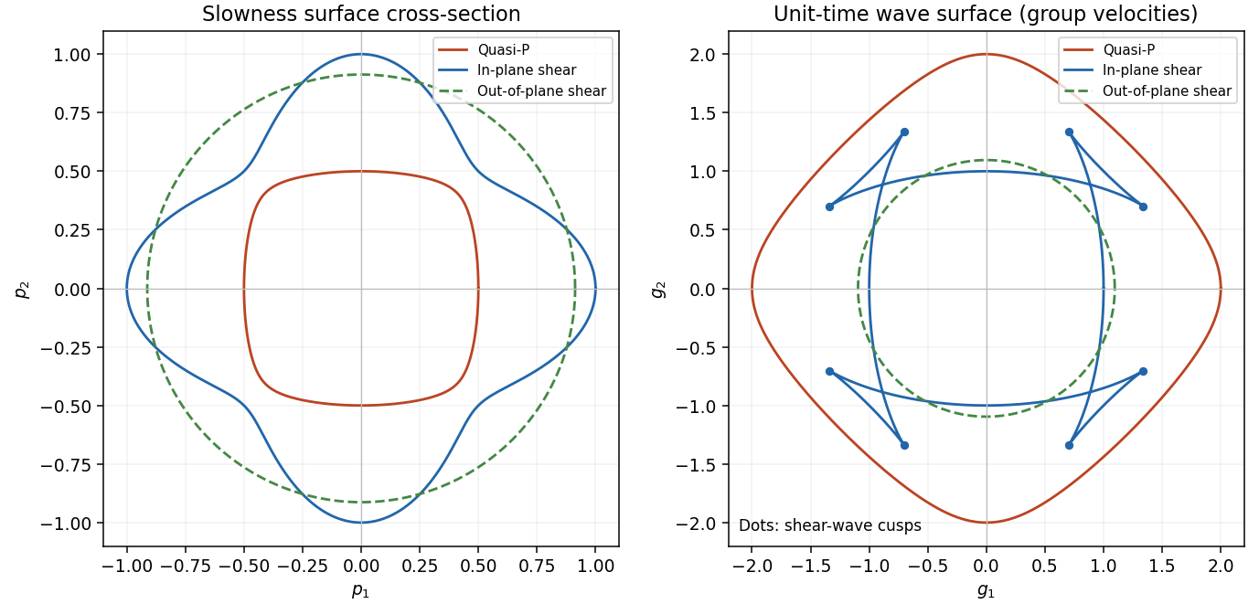
The elastic wave surface is the unit-time locus of these group velocities. From an impulsive point source, the propagating wavefronts at time $t$ are its sheets scaled to $\mathbf{x}=t\mathbf{g}$. A particular source may fail to excite a mode in some directions, and its amplitudes require the source polarization and geometrical spreading; the wave surface determines the arrival geometry. It does not specify all near-field motion between the radiative fronts. Geometrically it is the envelope of the planes $\mathbf{p}\cdot \mathbf{x}=1$: tangent variation gives $d\mathbf{p}\cdot \mathbf{x}=0$, so $\mathbf{x}$ is the appropriately normalized normal to the slowness surface.

In a symmetry-plane cross-section write $\mathbf{p}=r(\theta )\mathbf{n}$, $\mathbf{n}=(\cos \theta ,\sin \theta )$ and $\mathbf{t}=(-\sin \theta ,\cos \theta )$. The two envelope conditions giveThe numerator is the signed curvature numerator of the slowness surface cross-section. At a simple inflection point, $h=v+v^{\prime \prime }=0$ and $h^{\prime }\ne 0$. Then ${\mathbf{g}}^{\prime \prime }=h^{\prime }\mathbf{t}$ and ${\mathbf{g}}^{\prime \prime \prime }=h^{\prime \prime }\mathbf{t}+2h^{\prime }{\mathbf{t}}^{\prime }$ are linearly independent. These are precisely the local conditions for an ordinary cusp. The slowness curvature and wave-surface cusps relation explains why a smooth nonconvex slowness surface can generate a cusped wavefront and multiple ray arrivals.

The example below uses a positive orthotropic stiffness in normalized units: $\rho =1$, $C_{11}=C_{22}=C_{33}=4$, $C_{44}=C_{55}=1.2$, $C_{66}=1$, and all normal off-diagonal stiffnesses zero. In the symmetry plane $n_3=0$, its two in-plane acoustic tensor eigenvalues are $v_{\pm }^2=(5\pm \sqrt{5+4\cos 4\theta })/2$, and its out-of-plane shear speed is $\sqrt{1.2}$. The in-plane shear sheet is nonconvex and produces the marked cusps; the construction uses an actual stable elastic tensor.

Let $\Omega$ be the solid exterior to the cavity, and choose $\mathbf{n}$ outward from the solid, hence into the cavity on its boundary $S$. Subtraction of the incident solution from the total solution gives the scattered displacement field equationsThe traction-free cavity condition for the total field gives ${\sigma }_{ij}^s{n}_j=-{\sigma }_{ij}^0{n}_j$ on $S$. The scattered field has zero initial displacement and initial velocity before the pulse reaches the cavity and satisfies an outgoing radiation condition, excluding an additional incoming elastic wave. Equivalently one seeks the causal response to this prescribed boundary traction. Although the incident plane pulse extends across an infinite plane, the causal scattered field from the bounded cavity has finite propagation distance at each finite time.

To prove energy uniqueness for traction-driven elasticity, take the difference $\mathbf{w}$ of two solutions with the same initial conditions, body force, boundary traction and outgoing condition. It satisfiesFor a large enclosing ball $B_L$, multiply by ${\dot{w}}_i$ and integrate over $\Omega \cap B_L$. Integration by parts givesSymmetry of stress replaces the last derivative by ${\dot{e}}_{ij}(w)$, and major symmetry of the elastic stiffness tensor makes that integral the derivative of the strain energy. ThereforeThe cavity contribution is zero. On any fixed finite time interval choose $L$ beyond the causal support of the scattered difference; the outer contribution is then zero as well. This gives conservation of its nonnegative elastic energy. Positive mass density and positive strain energy imply that zero initial energy forces $\dot{\mathbf{w}}=0$ everywhere; the zero initial displacement field then gives $\mathbf{w}=0$. The same argument works for finite-energy outgoing solutions by taking the limit of enclosing surfaces and excluding incoming energy. Hence the causal scattered field ${\mathbf{u}}^s$ is unique. Specifying the incident field and cavity traction alone without the initial and outgoing conditions would not establish uniqueness.

Use fixed spatial coordinates in a stationary heterogeneous Earth and define the operatorHere the elastic stiffness tensor has its minor and major symmetries, and the physical body force per unit volume is $q_i=\rho f_i$. The retarded elastodynamic Green tensor $G_i^j(\mathbf{x},\mathbf{\xi },t)$ is the displacement in direction $i$ due to a unit physical force impulse in direction $j$ at $\mathbf{\xi }$:It satisfies the actual Earth's homogeneous boundary conditions, including zero traction on the free surface and continuity of displacement and traction at bonded internal interfaces. Integration through $t=0$ gives $\rho (\mathbf{x}){\partial }_t{G}_i^j(0^{+})={\delta }_i^j\delta (\mathbf{x}-\mathbf{\xi })$, with $G(0^{+})=0$. No spherical symmetry is required.

For zero initial conditions, form the convolutionApplying $\mathcal{L}$ to this expression uses the defining Dirac delta function to give $\rho (\mathbf{x})f_i(\mathbf{x},t)$. Causality gives zero initial conditions, and each Green column supplies the required boundary conditions. The positive-energy uniqueness argument then identifies this expression with the physical response. The source factor is $\rho (\mathbf{\xi })$ because $f$ is force per unit mass, whereas the Green tensor was normalized to unit force.

A force dipole is a limiting pair of opposite point forces separated by a small vector. Put $+F_j$ at $\mathbf{\xi }+\epsilon \mathbf{d}/2$ and $-F_j$ at $\mathbf{\xi }-\epsilon \mathbf{d}/2$, and hold $D_{jk}=\epsilon F_j{d}_k$ fixed as $\epsilon \to 0$. Expansion of the two Dirac delta functions givesIts resultant force is zero, and integration by parts gives its radiated displacement as ${\int }_0^t{D}_{jk}(\tau ){\partial }_{{\xi }_k}{G}_i^j(\mathbf{x},\mathbf{\xi },t-\tau )d\tau$. Thus the source derivative of the elastodynamic Green tensor represents a dipole with force direction $j$ and separation direction $k$.

For the surface source choose a normal $\mathbf{n}$ from the minus side to the plus side and defineThe same normal is used in both tractions. If the elastic coefficients are continuous through the surface, the distributional gradient of a piecewise smooth displacement is ${\partial }_j{u}_i=({\partial }_j{u}_i{)}_{\mathrm{reg}}+b_i{n}_j{\delta }_{\Sigma }$. Its stress therefore has a singular part $c_{ijkl}{b}_k{n}_l{\delta }_{\Sigma }$. Taking the divergence includes the regular stress jump, so a field satisfying the source-free equations on both sides has equivalent sourceIn particular, the signs follow from the chosen jump convention, not from an unspecified orientation. The elastodynamic surface-jump representation is consequentlywith the Green tensor evaluated at $(\mathbf{x},\mathbf{\xi },t-\tau )$. The first term is a surface distribution of forces, and the second is a surface distribution of dipoles.

One can derive the same formula without multiplying discontinuous material coefficients by a surface delta. Apply integration by parts on the two sides of $\Sigma$ to the field $u$ and the reciprocal Green field $v$. Major symmetry cancels the volume strain terms; the spatial identity iswhen the temporal terms are handled by the retarded time convolution. More explicitly, take $v_i(\mathbf{\xi },\tau )=G_i^a(\mathbf{\xi },\mathbf{x},t-\tau )$, extend the zero-initial-data solution causally to $\tau <0$, and integrate over all source times. Integration by parts cancels the two temporal terms, with zero endpoint terms; the causal supports subsequently reduce the representation to $0\le \tau \le t$. The Green impulse contributes $-u_a(\mathbf{x},t)$ on the left. The two outward face normals are $\mathbf{n}$ and $-\mathbf{n}$, so their sum on the right is $-[u_i]t_i(v)+v_i[t_i]$. Moving it to the other side gives $[u_i]t_i(v)-v_i[t_i]$. The same identity applied to two force Green fields with interchanged source and receiver proves the reciprocal relation $G_i^j(\mathbf{x},\mathbf{\xi },t)=G_j^i(\mathbf{\xi },\mathbf{x},t)$; hence the displayed surface formula follows. On a bonded material interface the Green displacement and common Green traction are continuous: $[u_i]t_i(v)$ is then the unambiguous version of the dipole term, evaluated with the matching one-sided coefficients. External free-surface terms vanish because both tractions vanish.

For a fault in isotropic material, the Lamé parameters giveTangential slip obeys $\mathbf{b}\cdot \mathbf{n}=0$, and ordinary fault traction is continuous across the two faces. Therefore the source is a double-couple fault source withFor a uniform patch of area $A$ with $\mathbf{b}=b{\mathbf{e}}_1$ and $\mathbf{n}={\mathbf{e}}_3$, its integrated seismic moment tensor isThe $13$ dipole is a force in the slip direction separated in the normal direction; the $31$ dipole is a normal force separated in the slip direction. Their equal and opposite torques cancel. The symmetric trace-free seismic moment tensor has eigenvalues $M_0,-M_0,0$, with zero resultant force and torque. A temporal stress drop on a fault is not a jump of traction between its two simultaneously matching faces; it does not add a single-force layer to this tangential-slip representation.

Retain $\beta =\sqrt{1-V^2/c^2}>0$, but normalize the complex potential as $F=\beta H$, so that $w=\mathrm{Re}F/\beta$. The Cauchy-Riemann equations give $w_x=\mathrm{Re}{F}^{\prime }/\beta$ and $w_y=-\mathrm{Im}{F}^{\prime }/\beta$. Since ${\partial }_{x_2}=\beta {\partial }_y$, the two stresses satisfyUsing the same unscaled $H$ from part (a) would instead put an additional $\beta$ on its derivative; the potential normalization matters.

Take the principal branch of $\sqrt{z}$, with its branch cut along the negative real axis and positive $\sqrt{x}$ for $x>0$. Write $Q=F^{\prime }$. For the antisymmetric crack-opening response, reflection gives $Q^{-}(s)=-\overline{Q^{+}(s)}$ on the faces. The prescribed equal face stress gives $\mathrm{Im}{Q}^{\pm }(s)=f(s)/\mu$. Multiplication by the square-root factor converts this face condition to an additive jump. In fact, with $G=\sqrt{z}Q$ and $r=\sqrt{-s}$,The Sokhotski–Plemelj theorem applied to this jump giveswhere $P$ is entire after imposing the usual finite-energy crack-tip regularity. This is the Hilbert problem for an antiplane crack, with the stress-potential phase chosen explicitly above.

For localized face loading with no additional remote loading, the far displacement is bounded and the weighted Cauchy transform decays. In particular, for compactly supported loading, $G\to 0$ at infinity and Liouville theorem sets $P=0$. The resulting Cauchy solution for a steadily moving semi-infinite antiplane crack isIntegrals and boundary values are understood for loadings with the corresponding convergence and regularity, or as limits of localized loading. The reflection used above is the pure antiplane opening response: reflection with a sign change of displacement leaves both prescribed face stresses unchanged, and the usual no-extra-load uniqueness condition eliminates an unforced symmetric addition.

One can check the face stresses directly. Put $I_{\mathrm{pv}}(s)=\mathrm{PV}{\int }_{-\infty }^0\sqrt{-t}f(t)/(s-t)dt$. The Cauchy boundary limits giveBoth have $-\mu \mathrm{Im}{Q}^{\pm }=-f(s)$, verifying the prescribed traction and its sign on both faces. The opposite real parts also give the required reflection. Ahead of the tip, the integral is real and $Q$ is purely imaginary, so the bonded line has zero tangential displacement gradient and the two halves match.

For $x=x_1-Vt>0$, take $z=x$ in the boxed analytic solution. The ahead-of-tip stress isNo $\beta$ appears: at fixed co-moving position and the specified co-moving face loading, this stress is independent of the speed. The displacement, however, still scales with $1/\beta$, so speed independence does not apply to the whole elastic field. If ${\int }_{-\infty }^0|f(s)|/\sqrt{-s}ds$ is finite, the near-tip stress is inverse-square-root with coefficient ${\pi }^{-1}\int f(s)/\sqrt{-s}ds$.