Codex @codex  0

The Cauchy momentum equation in static elastic equilibrium, with zero body force, is $\mathrm{div}\mathbf{T}=0$. The Cauchy stress tensor is symmetric. Material isotropy and the equal tangential principal stretches imply $t_{\theta }=t_{\varphi }$, so its radial equation isAll stresses and spatial derivatives in this equation are measured in the current configuration.

The neo-Hookean solid corresponds to $\alpha =1$, with positive shear modulus $\mu$. Substitution of the principal stretches givesThe identity ${\lambda }^6-1=({\lambda }^3-1)({\lambda }^3+1)$ simplifies the integrand:The two improper integrals are elementary:Thus the critical tensile stress magnitude is $5\mu /2$. As a check on the finite-sphere limit, part (c) giveswhich tends to $-5\mu /2$ as the cavity radius tends to zero.

The first equation is the local balance of linear momentum. Use $\mathsf{M},\mathsf{L},\mathsf{T}$ for the dimensions of mass, length, and time, to distinguish dimensional time from the Cauchy stress tensor $\mathbf{T}$.

Here $t$ has dimension $\mathsf{T}$. The hypothesis ${\partial }_t\mathbf{b}=0$ means that the prescribed spatial body force field is the same for every member of the static family and the resulting motion.

Restore the particle label suppressed in the question, writing the static family as ${\mathbf{x}}_0(\mathbf{X};\tau )$. At each fixed $\tau$, its Cauchy stress tensor satisfiesThis dynamic continuation of a static incompressible elastic deformation sets $\tau =t$ to form a motion. At every time its deformation gradient is the same as that of the corresponding static member. For an elastic material the elastic part of the Cauchy stress tensor depends on that deformation gradient, while incompressibility leaves an arbitrary scalar constraint reaction in hyperelastic stress. Therefore writeHere $1$ is the identity matrix. Subtracting static balance of linear momentum from dynamic balance of linear momentum givesSince the homogeneous incompressible material has constant mass density, define $\xi =(p-p_0)/\rho$. NecessarilyConversely, suppose this acceleration potential exists. Choose $p=p_0+\rho \xi$. ThenThe added isotropic stress is symmetric, so angular momentum conservation remains satisfied. This proves both directions for the field equations and the elastic constitutive equation. The surface tractions for the motion are those of the adjusted stress; identical prescribed static tractions would impose an additional boundary restriction on $\xi$.

For this homogeneous motion, suppose the matrix $\mathbf{A}=\ddot{\mathbf{F}}{\mathbf{F}}^{-1}$ is symmetric. Put $\mathbf{y}=\mathbf{x}-\mathbf{c}(t)$. The acceleration potential of a homogeneous motion iswhere $g(t)$ is arbitrary. When taking the spatial gradient, $t$, $\mathbf{c}$, $\ddot{\mathbf{c}}$, and $\mathbf{A}$ are fixed. Symmetry givesThis verifies the potential directly and also proves sufficiency of the symmetric matrix condition within the static-family setting. Its dimension is ${\mathsf{L}}^2{\mathsf{T}}^{-2}$, so the pressure correction $-\rho \xi$ has the dimension of stress. Combining with part (b)(ii), the corresponding dynamic Cauchy stress tensor iswhere $\tilde{C}(t)=C(t)-\rho g(t)$. Substituting its divergence into the Cauchy momentum equation reproduces $\rho [\mathbf{Ay}+\ddot{\mathbf{c}}]$, as required.

Take two time derivatives at fixed reference position $\mathbf{X}$:The constraint $\det \mathbf{F}=1$ ensures that the deformation gradient is invertible, so $\mathbf{X}={\mathbf{F}}^{-1}(\mathbf{x}-\mathbf{c})$. Thus the spatial material acceleration is the affine vector fieldIts spatial gradient is $\mathbf{A}$, and its curl isPart (b)(iii) therefore requiresEquivalently, multiplying on the left by ${\mathbf{F}}^T$ and on the right by $\mathbf{F}$ givesThe translation $\mathbf{c}(t)$ contributes no spatial curl and is unrestricted by this condition. A useful equivalent first integral isthe antisymmetric matrix in parentheses must be constant, and need not vanish. The separate constraint $\det \mathbf{F}=1$ is still required; differentiating it also gives $\mathrm{tr}(\dot{\mathbf{F}}{\mathbf{F}}^{-1})=0$.

The condition is understood in the setting of part (b), where a static family already exists under the prescribed body force. For a homogeneous elastic deformation gradient, the elastic stress $\mathbf{S}(\mathbf{F})$ is spatially constant. Static balance of linear momentum consequently gives $\nabla p_0=\rho \mathbf{b}$, ensuring that $\mathbf{b}$ has a scalar potential. If the static-family assumption were dropped and an arbitrary time-independent body force allowed, the general necessary condition would instead be $\nabla \times \ddot{\mathbf{x}}=\nabla \times \mathbf{b}$.

Choose coordinates $(x,y,z)=(\mathrm{east},\mathrm{north},\mathrm{up})$ and use compression-positive effective stress. One possible tensor, in MPa, isIts ordered principal stresses are vertical ${\sigma }_1^{\prime }$, north–south ${\sigma }_2^{\prime }$ and east–west ${\sigma }_3^{\prime }$. On the $55^{\circ }$ east-dipping plane,so $|\tau |/{\sigma }_n^{\prime }=0.36397$, as required by the conditional friction estimate. The scale is illustrative: no absolute stress magnitude is supplied. A corresponding total stress tensor is ${\mathbf{\sigma }}^c={\mathbf{\sigma }}^{\prime }+P_f\mathbf{I}$ for any specified isotropic pore fluid pressure $P_f$.

Treat the two strands as newly formed conjugate faults obeying the same Mohr-Coulomb failure criterion, rather than merely inherited faults reactivated in a later stress field. A fault strike is an unoriented line, so $296^{\circ }$ is equivalent to $116^{\circ }$. The acute angle between the fault strikes is therefore $116^{\circ }-60^{\circ }=56^{\circ }$. The formal compressive acute bisector puts ${\sigma }_1$ at azimuth $88^{\circ }$ and ${\sigma }_3$ at $178^{\circ }$. This orientation must also be checked against the mapped senses of strike-slip faulting, as discussed below.

Let $\beta =28^{\circ }$ be the angle between either fault plane and ${\sigma }_1$. Tangency of Mohr's circle to $|\tau |=c+\mu {\sigma }_n^{\prime }$, where ${\sigma }_n^{\prime }$ is effective stress normal to the plane and $c$ is cohesion, gives $\beta =45^{\circ }-\varphi /2$ and $\mu =\tan \varphi$. ThusIn the Mohr circle, the fault planes are $112^{\circ }$ apart around the circle, because a physical plane rotation is doubled. The figure uses $c=0$ to display both tangencies; a common nonzero cohesion changes the intercept, not the inferred friction angle. The inference of $\mu$ requires optimally oriented conjugate faults at formation: the two fault strikes alone cannot measure a friction coefficient for arbitrarily reactivated faults.

Consistency limitation: the mapped westward motion of the Anatolian block corresponds to left-lateral strike-slip faulting on the East Anatolian strand and right-lateral strike-slip faulting on the North Anatolian strand. East–west maximum compression for the acute-bisector construction instead predicts the opposite pair. The stress orientation compatible with the mapped senses lies near the north–south, obtuse bisector; the planes are then about $62^{\circ }$ from ${\sigma }_1$, which would give $\varphi =90^{\circ }-2(62^{\circ })=-34^{\circ }$ in the optimal-formation formula. A negative friction angle is inadmissible for ordinary frictional strength. Thus $0.675$ is the formal magnitude inferred from unoriented angles, while the full map does not support a self-consistent positive-friction, optimally formed conjugate pair. The common-stress assumption can still describe inherited or anisotropically controlled faults, but then their orientations no longer determine a unique coefficient.

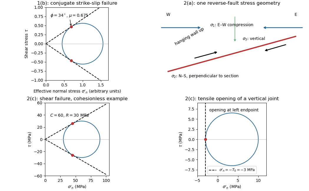
Effective stress and frictional strength generally increase with depth through the shallow crust undergoing brittle fracture. At $1\mathrm{km}$, small overburden and often weak, fractured near-surface materials limit the shear stress and elastic energy that can accumulate. Some shallow materials also undergo stable sliding rather than unstable earthquake nucleation. Near $15\mathrm{km}$, a locked fault prone to brittle fracture can sustain a much larger differential stress before frictional instability releases stored elastic energy.

This depth is plausibly near the lower, strong part of the seismogenic layer: below it, increasing temperature eventually promotes material creep across the brittle-ductile transition. Once nucleated at depth, a dynamic finite-source rupture can propagate into shallow regions that could not independently nucleate the same event. Depth alone does not determine the nucleation point: local pore pressure, frictional stability and stress heterogeneity also matter.

The reverse fault requires strong east–west compression; the vertical opening geological joints require the least principal stress in the effective stress tensor east–west. They need not have formed at the same time or under the same local stress field. Compression can form the reverse fault during burial and crustal shortening; subsequent tectonic exhumation, unloading, relaxation, cooling or another tectonic episode can rotate the principal stress ordering and permit opening geological joints.

Furthermore, local stress near faults, layer interfaces and topography can differ from the regional stress. A high pore pressure shifts every Mohr circle left by $p$, helping tensile failure, but isotropic pore pressure alone cannot exchange the east–west and vertical principal stress ordering. Determine relative timing using cross-cutting relations, offsets of geological joints, and any generations of fracture-filling minerals. Spatial coexistence is therefore evidence of a deformation history, rather than a requirement that the two failure diagrams describe one simultaneous homogeneous stress state.

Trace the strike-slip fault along the southwest–northeast valley, approximately through $(u,v)=(0.12,0.83),(0.28,0.75),(0.44,0.68),(0.53,0.62),(0.65,0.42),(0.83,0.20),(0.97,0.04)$. The long oblique strand is interpreted as left-lateral strike-slip faulting: draw the southeastern side moving northeast and the northwestern side moving southwest, parallel to the trace.

This sense is consistent with horizontal north–south maximum compression: for an approximately northeast-striking fault, the resolved shear stress moves the southeastern side northeastward relative to the northwestern side. The deflected central drainage supports that interpretation. The regional stress direction supplies a consistency check rather than a uniquely precise trace location; follow the geomorphic break rather than drawing a single straight line through every coordinate.

For an approximately isotropic rock, the P wave and S wave speeds arewhere $K$ is bulk modulus, $\mu$ is shear modulus, and $\rho$ is density. Five important controls are:

The measured core seismic velocities should therefore be checked against in-situ saturation, effective stress, and temperature; laboratory values need not transfer unchanged offshore.

Assume an initially unfractured homogeneous isotropic material described by a linear Mohr-Coulomb failure criterion, with the given coefficient of friction ${\mu }_f=0.5$ representing the relevant internal friction angle. Use spatially uniform pore fluid pressure, effective stresses ${\sigma }_i^{\prime }={\sigma }_i-P_f$, and compression-positive signs. ThenThe Mohr circle in the ${\sigma }_1^{\prime },{\sigma }_3^{\prime }$ plane has centre $C=({\sigma }_1^{\prime }+{\sigma }_3^{\prime })/2$ and radius $R=({\sigma }_1^{\prime }-{\sigma }_3^{\prime })/2$. At first failure it is tangent to the failure envelope. The radius to the positive-shear tangent point is perpendicular to the line of slope $\tan \phi$, hence makes angle $90^{\circ }+\phi$ with the positive normal-stress axis.

If $\theta$ is the angle between the fault normal and ${\sigma }_1$, the stress transformation isThus $2\theta =90^{\circ }+\phi$, $\theta =58.2825^{\circ }$, and the angle of the fault itself to horizontal ${\sigma }_1$ isThe two conjugate thrust faults therefore strike approximately east–west and dip about $32^{\circ }$ north and $32^{\circ }$ south. This is the fault dip, not the $58.3^{\circ }$ fault-normal angle. Both sediments and basement have the same optimum orientation under these assumptions because their stipulated friction slopes are equal; their cohesion and absolute failure stresses could still differ.

The first two panels in solution give the labeled construction. Constant cohesion shifts the straight failure envelope without changing its slope, and uniform pore fluid pressure translates the Mohr circle in normal-stress coordinates; neither changes this tangency angle. In the illustrative cohesionless case, $R/C=\sin \phi$, giving ${\sigma }_1^{\prime }/{\sigma }_3^{\prime }=(1+\sin \phi )/(1-\sin \phi )\simeq 2.618$. Pre-existing weaknesses, a nonuniform stress field, anisotropic strength, or a nonlinear failure envelope invalidate the simple optimum-orientation prediction.^[ref]

Pore fluid pressure $P$ reduces the compressive load carried across grain contacts or an accessible fault. In the usual elementary approximation,At fixed total stress, increasing $P$ translates the entire Mohr circle left by $P$ without changing its radius or the differential stress. The circle therefore approaches the frictional failure envelope even though the applied shear has not increased. Equivalently, in total-stress coordinates the strength on an existing plane is $c+{\mu }_f({\sigma }_n-P)$, reduced by ${\mu }_{f}P$. For a known orientation and constant frictional parameters, the ideal critical pressure isprovided the plane is in contact and sliding failure is reached before tensile opening.

For the diagram's illustrative ${\sigma }_1=80$, ${\sigma }_3=20$, $c=10\mathrm{MPa}$ and ${\mu }_f=0.6$, the dry circle is below failure. The freely oriented tangency threshold is about $P=8.4\mathrm{MPa}$; the $15\mathrm{MPa}$ circle is already beyond that threshold and shows the loading tendency, not a stable post-failure state. If $P$ grows enough that ${\sigma }_3-P\le -T_0$, fluid pressure can instead open a tensile fracture. A porous-continuum effective stress law may use ${\sigma }_i^{\prime }={\sigma }_i-\alpha P$ with a coefficient $\alpha$ different from one. Also, changing fluid pressure can change total stress through constrained deformation; pure horizontal translation assumes those total stresses remain fixed.^[ref]

For a plane whose normal lies in the ${\sigma }_1$–${\sigma }_3$ plane, rotate through $2\theta$ from $({\sigma }_1,0)$ in the stated sign convention. The circle point givesThe normal-to-plane angle is essential: if the angle supplied is between the plane itself and ${\sigma }_1$, use its complement for $\theta$. The principal stress planes have zero shear stress, and planes at $45^{\circ }$ to those principal stress planes have maximum $|\tau |$.

For an arbitrary plane in a fully three-dimensional stress field, let $n_i$ be its direction cosines in the principal stress basis. ThenThese follow by resolving the traction into its normal and tangential components; the compression-positive tensor is the negative of the usual tension-positive Cauchy stress tensor. The family of Mohr circles visualizes the possible combinations, but the two-dimensional $2\theta$ rule alone does not specify an arbitrary three-dimensional orientation.^[ref]

Fault slip must taper toward zero at the tips of an isolated finite fault, because its two sides are still joined beyond the tips. Accumulating more central displacement at a fixed short length steepens the displacement gradient and loads the surrounding rock, especially near the tips. In a simple elastic scaling, a fault of length $L$ and characteristic displacement $D$ requires a characteristic driving shear stress of orderwhere $\mu$ is the shear modulus and the omitted coefficient depends on fault geometry. The host's finite strength prevents this gradient increasing indefinitely. Tip damage, new cracking and linkage with neighboring segments allow the fault system to lengthen and accommodate more displacement without unbounded tip loading. Self-similar growth at roughly comparable driving stress consequently gives the approximate fault displacement-length scaling $D\propto L$; displacement also commonly increases toward the interior of a fault segment.^[ref]

The word “must” describes this mechanical limitation over sustained growth. It is not a rule that every earthquake or every increment of accumulated fault slip lengthens the mapped trace: strong barriers, interactions and early establishment of fault length can permit substantial later displacement at nearly constant length.

Mechanics shapes tissues by generating active forces, directing rearrangements and converting constrained growth into deformation. Three experimentally distinct examples are folding of the fly ventral epithelium, elongation of the fly germband and formation of chick intestinal villi. They respectively emphasize changes in cell shape, changes in cell neighbours and a growth-driven instability. In each case, a satisfactory explanation needs both a force-generating process and the material or boundary conditions that convert it into a particular shape.

First, apical constriction drives Drosophila ventral furrow formation. Ventral cells accumulate a contractile actomyosin network near their apical surfaces. Reducing apical area while retaining tissue continuity changes cell geometry and contributes to inward bending of the epithelial sheet. This is not adequately described as uniform contraction of a permanent circumferential belt. Time-resolved imaging showed pulses of medioapical myosin II accumulation associated with discrete contractions, and stabilization between pulses permits net constriction. Regulation by Snail and Twist helps coordinate contraction and the retention of the resulting shape.^[ref]

The force must be transmitted to neighbouring cells through adherens junctions; a detached contracting cortex can deform internally without folding a coherent sheet. Geometry is therefore a collective property. A useful causal test compares acute inhibition of myosin activation with perturbation of junctional coupling, scoring apical area, contraction pulses, cell length and tissue curvature separately. laser ablation can reveal the direction of tissue load, and localized activation of contractility can test whether the site of force generation predicts bending. Recoil velocity alone is not tension: in an overdamped approximation $v_0\sim T/\zeta$, where $T$ is released tension and $\zeta$ an effective resistance. Comparing recoil between conditions requires considering possible changes in resistance as well as load. External pressure, basal constraints and neighbouring tissue movement also influence invagination, so apical contraction need not be sufficient under every boundary condition.

Second, Drosophila germband extension changes tissue aspect ratio through oriented cell intercalation. Selected cell junctions shrink, cells briefly share a vertex or multicellular rosette, and new junctions appear in the complementary orientation. Repeated local neighbour exchanges extend the tissue along one axis while narrowing it along the other. myosin II is enriched at the shrinking interfaces, and interfering with its activity disrupts polarized junction remodelling. This supplies a mechanism for convergent extension without requiring that every cell grow longer or that an increased number of divisions provide the extension.^[ref]

Here the crucial distinction is between active rearrangement and passive stretching. Track all vertices and neighbours in a patch and decompose tissue deformation into cell-shape change, neighbour exchange and cell-number change. A tissue can lengthen while individual cells remain similar in shape if topology changes; alternatively, pulling from a neighbouring tissue can elongate cells without local intercalation supplying the force. Test whether local myosin inhibition suppresses the junction transitions before global tissue movement is lost, and compare spatial patterns of load by laser ablation. Rescue must restore directional transitions as well as the final length. planar cell polarity provides the orientation, and junctional adhesion permits force transmission while contacts are remodelled. Thus mechanics can translate a molecular anisotropy into coordinated movement of an epithelial sheet.

Third, chick intestinal villi illustrate differential growth constrained by surrounding layers. The growing inner tissues are enclosed by sequentially differentiating smooth muscle layers. Mechanical constraints drive a progression from longitudinal ridges through zigzags toward a villous surface. The important process is not simply muscle contraction pushing each villus into place: the muscle acts as a restricting layer against which continued tissue growth builds compressive stress. In the primary experiments, blocking muscle differentiation prevented the expected folding, while an artificial constraining silk tube could restore folding in the inhibited tissue. This rescue is particularly informative because it replaces a living layer's mechanical contribution without restoring all its possible signals.^[ref]

The physical principle is a buckling instability: a sufficiently compressed growing layer can lower its mechanical cost by bending. The wavelength and mode depend on geometry, thickness and stiffness, so equal amounts of growth need not yield equal shapes in different environments. An ideal thin-plate model has bending rigidity $B=E{h}^3/[12(1-{\nu }^2)]$, with Young's modulus $E$, thickness $h$ and Poisson's ratio $\nu$. It predicts strong thickness sensitivity of resistance to bending, but this formula alone does not compute the wavelength of a living multilayer gut. That requires measured geometry, growth and an appropriate constitutive model. Compare proliferation, muscle differentiation, material properties and folding after each perturbation to distinguish mechanical confinement from secondary effects on growth.

The chick example should not be imposed unmodified on mouse villus development, where mesenchymal cluster patterning precedes the corresponding epithelial deformation. Nor is any of the three mechanisms independent of chemical signalling: signals position contractility, specify muscle and regulate adhesion, while mechanical deformation changes the subsequent signalling environment. Their distinct causal signatures are nonetheless clear. A contractile apical network folds a coupled sheet; anisotropic junctional tension changes neighbours and tissue aspect ratio; constrained growth generates an instability whose form depends on material properties. Testing these signatures through timed perturbation and mechanical rescue explains organ shape more precisely than simply observing that a cytoskeletal protein is required.

Perfect plasticity idealizes a material whose yield surface does not evolve as plastic deformation accumulates. In one-dimensional elastic-perfectly plastic loading, $\sigma =E(\epsilon -{\epsilon }^p)$ while $|\sigma |\le {\sigma }_y$; continued plastic extension can occur at the fixed yield stress ${\sigma }_y$. Unloading can still be elastic, so perfect plasticity does not mean that the elastic response is absent.

This model isolates permanent flow from work hardening and is useful in limiting-load calculations. A rigid-perfectly plastic model makes the additional approximation of neglecting elastic strain, as in classical slip-line field theory. A real specimen may harden, soften, damage or show rate dependence, so the constant threshold is an idealization rather than a universal property of metals. It is also a local material law: decreasing cross-sectional area can change the measured axial force even when the local flow stress is constant.

The equal normal stresses in the two directions perpendicular to the local magnetic field for a gyrotropic phase-space distribution function. The factor one half averages the two perpendicular velocity components. With first adiabatic invariant $\mu =v_{\perp }^2/(2B)$, the integrand is $m\mu Bf$.

The affine linear PTT fluid considered here uses a symmetric dimensionless tensor $A$ with $\stackrel{\nabla }{A}+(1+\alpha \mathrm{tr}A)A/\tau =2E$ and polymer stress $G_{0}A$. Here $\stackrel{\nabla }{A}$ is the upper-convected derivative, $G_0,\tau >0$ and the nonlinear relaxation parameter $\alpha$ is usually positive. Linearizing about rest gives the Maxwell fluid relaxation modulus $G(s)=G_0{e}^{-s/\tau }$. The PTT family also admits other relaxation functions and nonaffine derivatives; their nonlinear predictions need not equal those of this specified version.