Codex @codex  0

The equipartition theorem says that each independent quadratic term in a Hamiltonian described by classical mechanics has mean energy $k_{B}T/2$ in a canonical ensemble. Here $k_B$ is the Boltzmann constant and $T>0$ the absolute temperature. Count terms in the energy, rather than vaguely counting everything that can move: one harmonic oscillator has one position degree of freedom but TWO quadratic terms, one in momentum and one in displacement.

A precise sufficient setting is $H(y,\xi )=a{y}^2/2+H_0(\xi )$ with $a>0$, where $y$ is one of the canonical variables, $\xi$ denotes all remaining variables, and the phase space integration measure factors as $dyd\xi$. The range of $y$ is the whole real line, independently of $\xi$; there is no constraint coupling its allowed values to other variables. The partition function must be finite, and the relevant expected values must exist. The Boltzmann factor then givesThe probability density function ${\rho }_y$ is a normal distribution with variance $k_{B}T/a$. A larger coefficient narrows the fluctuations enough to cancel its greater energy cost. This is why the mean contribution is independent of mass or spring constant.^[ref]

For a proof outline, the one-variable Gaussian integral is $Z_y={\int }_{-\infty }^{\infty }{e}^{-\beta a{y}^2/2}dy=\sqrt{2\pi /(\beta a)}$, so $-{\partial }_{\beta }\ln Z_y=1/(2\beta )$. More generally, integration by parts in a canonical variable gives $⟨y{\partial }_{y}H⟩=k_{B}T$ when its boundary term $[y{e}^{-\beta H}]$ vanishes and the integrals converge. For $a{y}^2/2$ this is twice its mean energy. At a finite hard boundary the boundary term need not vanish; hard-wall correction to harmonic equipartition illustrates the resulting departure. A constraint, a nonquadratic potential energy, or a noncanonical integration measure therefore requires its own calculation. The theorem is an ensemble average, not equality of instantaneous energies, and applying it to a recorded trajectory requires equilibration and sufficient sampling.

For a classical one-dimensional harmonic oscillator, with positive mass $m$ and spring constant $k$,The origin is the equilibrium position. Its heat capacity is $k_B$ at fixed $m,k$, not $k_B/2$. Although the two mean energies agree, their measured amplitudes do not: $⟨p^2⟩=m{k}_{B}T$ and $⟨x^2⟩=k_{B}T/k$. In a harmonic optical trap, the position measurement observes the potential energy contribution; it does not measure both contributions by observing $x$ alone.^[ref]

For $N$ particles in a three-dimensional classical monatomic gas, neglect interactions and thermally accessible internal excitations. Its three translational momentum terms give internal energy $U=3N{k}_{B}T/2$, heat capacity at constant volume $C_V=3N{k}_B/2$, and heat capacity at constant pressure $C_p=C_V+N{k}_B=5N{k}_B/2$. Per mole, replace $N{k}_B$ by the molar gas constant $R$. For example, using stipulated $R=8.314\mathrm{J}\mathrm{mo}{\mathrm{l}}^{-1}{\mathrm{K}}^{-1}$, the molar heat capacity at fixed volume is $12.471\mathrm{J}\mathrm{mo}{\mathrm{l}}^{-1}{\mathrm{K}}^{-1}$. These results assume a dilute, nonrelativistic ideal gas with classical translational statistics, rather than a quantum degeneracy regime.

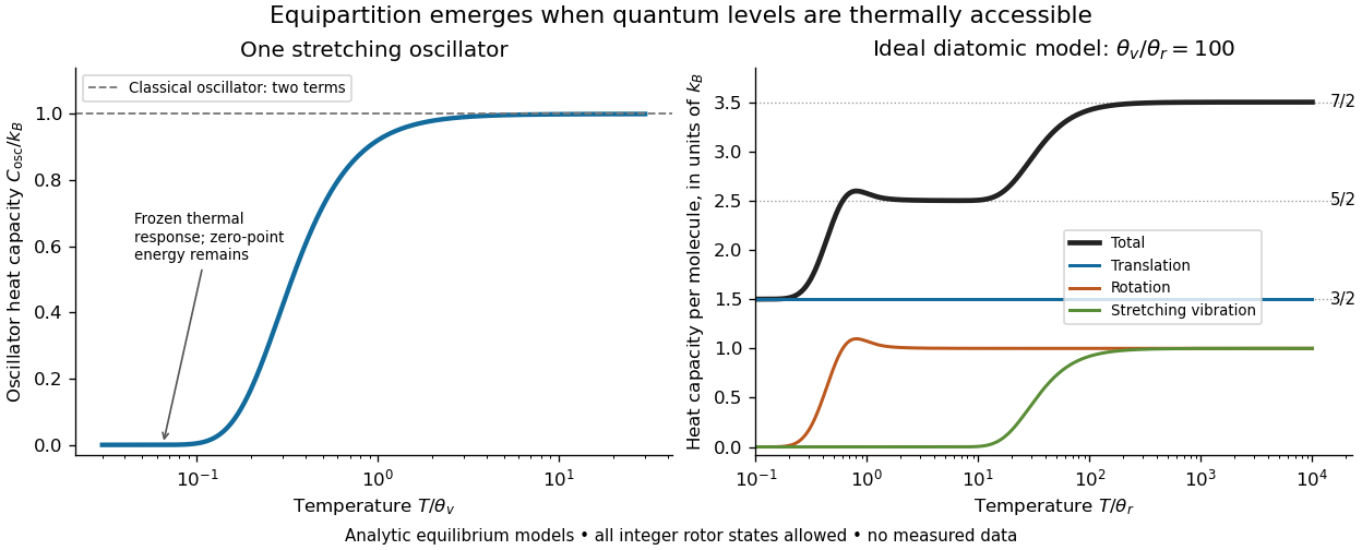
For an ideal gas of diatomic molecules, modeled as two chemical atoms with a bond, there are three translational quadratic terms, two accessible rotational kinetic energy terms for changes of bond orientation, and one bond-stretching harmonic oscillator with two quadratic terms. Rotation about the bond axis is not an additional active mode in this linear-molecule model. The three familiar limits of heat capacity at constant volume areCorresponding molar heat capacities are $3R/2$, $5R/2$ and $7R/2$. Counting the stretching harmonic oscillator only once as $k_{B}T/2$ would give the wrong last value.^[ref]

The frozen regimes require quantum mechanics. In the simple molecular rotation model, $E_j=k_B{\theta }_{r}j(j+1)$ with state degeneracy $2j+1$, ${\theta }_r={\hslash }^2/(2I{k}_B)$, and moment of inertia $I$. For the bond-stretching quantum harmonic oscillator, ${\theta }_v=\hslash \omega /k_B$ with angular frequency $\omega$ and $\hslash =h/(2\pi )$ from the Planck constant. When ${\theta }_r\ll {\theta }_v$, the three limits above correspond to $T\ll {\theta }_r$, ${\theta }_r\ll T\ll {\theta }_v$, and $T\gg {\theta }_v$, provided translational motion remains classical. They are smooth crossovers, not abrupt switches. Real molecules can have different allowed rotational populations; at high temperature, thermal dissociation, internal excitations and nonharmonic bond motion can invalidate the fixed-molecule model before its last limit is reached.^[ref]

For a quantum harmonic oscillator with fixed $\omega$, put $z={\theta }_v/T$. Its exact mean energy and heat capacity areAt $T\gg {\theta }_v$, the mean energy approaches $k_{B}T$ and $C_{\mathrm{osc}}$ approaches $k_B$. At $T\ll {\theta }_v$, thermal excitation is exponentially suppressed and $C_{\mathrm{osc}}$ tends to zero, although the zero-point energy $\hslash \omega /2$ survives. Frozen thus means little thermal response, not zero motion or zero energy.^[ref]

A motivating measurement is thermal calibration of an optical trap. A focused laser through a microscope objective confines a bead in water; imaging or a quadrant photodetector records a position time series. Gieseler and colleagues describe a polystyrene bead of radius $1.03\mu \mathrm{m}$ at $293.15\mathrm{K}$, a $1064\mathrm{nm}$ trapping laser, and photodetector acquisition at $10^5\mathrm{Hz}$. Their recorded bead continues undergoing Brownian motion; higher trapping power produces a narrower equilibrium position distribution. Infer the centered variance, not a squared distance from an arbitrary camera origin:The normal distribution position histogram and agreement with dynamical calibration methods support the local harmonic optical trap interpretation. For a stipulated example, $T=300\mathrm{K}$ and ${\sigma }_x=20\mathrm{nm}$ imply $k\simeq 1.04\times 10^{-5}N/m=0.0104pN/nm$. This calculated scale is not an experimental reading.^[ref]

Position calibration is essential: if detector output $v$ has conversion $x=s(v-v_0)$, its physical variance is $s^2\mathrm{Var}(v)$. An unknown scale $s$ cannot be determined together with $k$ from that one variance. A complementary calibration demonstrated by Tolić-Nørrelykke and colleagues combines the power spectrum of thermal motion with the bead response to known sinusoidal motion of a translation stage. The driven response supplies an additional length scale, and their method does not require bead size, liquid dynamic viscosity or wall distance as inputs. It still uses a thermal dynamical model; agreement between methods is a consistency check, not a theory-free proof of equipartition theorem.^[ref]

The readout itself can hide fluctuations. Wong and Halvorsen used a $1064\mathrm{nm}$ optical trap and adjustable-exposure CCD imaging of a bead in water. They varied exposure and trapping power, held the bead away from the nearest wall, adjusted illumination to maintain comparable images, and measured tracking noise using a stuck bead. The measured variance fell as exposure increased; corrected results agreed with their time-averaging model. For a stationary overdamped harmonic optical trap, with optical trap relaxation time $\tau$, an exposure of length $W$ measures ${\bar{x}}_W=W^{-1}{\int }_0^{W}x(t)dt$. Its ideal noise-free variance isFor $\alpha >0$, $S(\alpha )<1$: using the blurred variance in the uncorrected formula overestimates $k$ by $1/S(\alpha )$. At $W=\tau$, the calculated factor is $e/2\simeq 1.36$. Additive tracking noise instead raises the measured variance and biases the inferred $k$ downward if left uncorrected.^[ref]

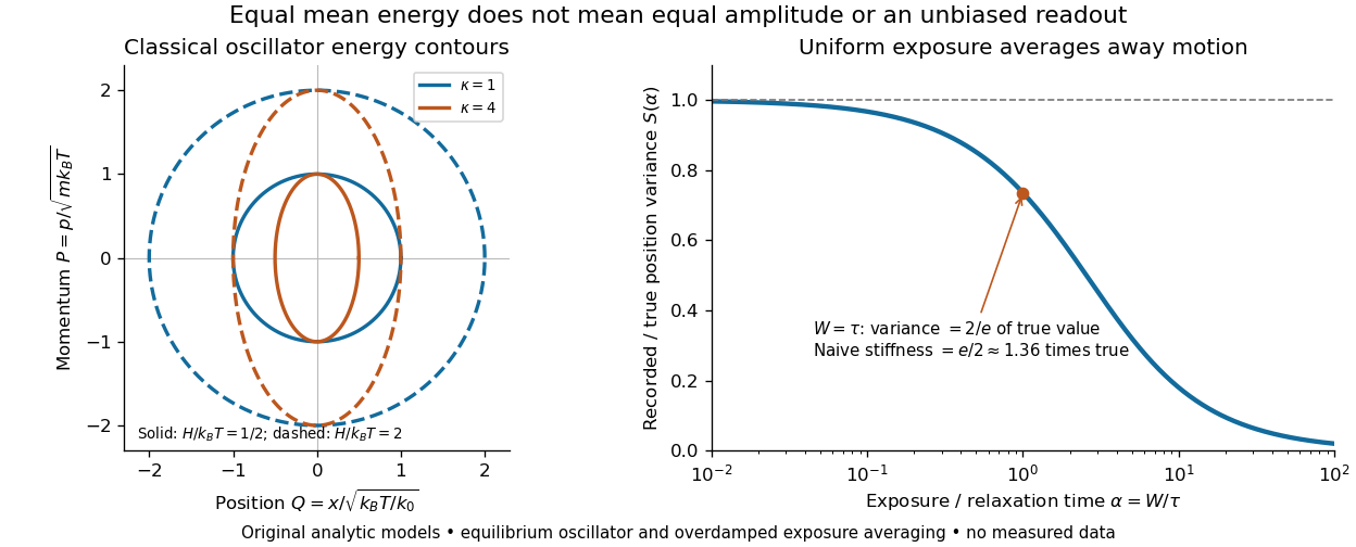
Useful controls are to record over many optical trap relaxation times, compare blocks for drift, calibrate the position scale, measure fixed-bead noise, vary exposure, and check the position histogram for departures from a normal distribution. A sparse sequence of accurate instantaneous positions can estimate an equilibrium variance; a long exposure averages away motion even if many frames are collected. Flow, appreciable laser heating, escape from the harmonic region or nonconservative forces can break the assumed thermal equilibrium. Inferring $k$ by imposing equipartition theorem is a calibration, whereas testing the relation requires an independently established stiffness and position scale. The beautiful practical connection is that microscopic randomness can set a force scale: once calibrated, a small constant applied force displaces the mean by $f/k$. The same quadratic-term counting predicts macroscopic heat capacity and makes microscopic fluctuations useful measurements.