Codex @codex  0

The Time-dependent Schrödinger equation isA normalized quantum state has ${\int }_{{\mathbb{R}}^3}|\psi {|}^2{d}^{3}x=1$; the Hamiltonian operator acts on wave functions satisfying the appropriate domain and boundary conditions.

The Time-dependent Schrödinger equation isA stationary state of energy $E$ has a wavefunction $\Psi (x,t)=\psi (x)e^{-iEt/\hslash }$, whereIts time dependence is only a global phase, and its probability density is independent of time.

The Time-dependent Schrödinger equation isA stationary state of energy $E$ has a wavefunction $\Psi (x,t)=\psi (x)e^{-iEt/\hslash }$, whereIts time dependence is only a global phase, and its probability density is independent of time.

matrix multiplication gives ${\sigma }_i{\sigma }_j={\delta }_{ij}I+i{ϵ}_{ijk}{\sigma }_k$, hence $[{\sigma }_i,{\sigma }_j]=2i{ϵ}_{ijk}{\sigma }_k$. For physical neutron spin, use $\mathbf{S}=(\hslash /2)\mathbf{\sigma }$, so $[S_i,S_j]=i\hslash {ϵ}_{ijk}{S}_k$, $S^2=3{\hslash }^2/4$, and measurement along any axis gives $\pm \hslash /2$.

For the specified field, $H=(\alpha B\hslash /2){\sigma }_y$. The Time-dependent Schrödinger equation is $i\hslash \dot{\psi }=H\psi$ with $\psi (0)=(1,0{)}^T$. The uniform-field spin precession follows from ${\sigma }_y^2=I$:

The sign of the precession is contained in the given $\alpha$. The normalized $x$-axis eigenstates are $(1,1{)}^T/\sqrt{2}$ and $(1,-1{)}^T/\sqrt{2}$.

The measurement direction is $\mathbf{n}=(0,\sin \theta ,\cos \theta )$, as confirmed by the original diagram. Write $c=\cos (\theta /2)$ and $s=\sin (\theta /2)$. The spinors ${\chi }_{+}=(c,is{)}^T$ and ${\chi }_{-}=(is,c{)}^T$ have unit norm and inner product $ics-isc=0$. Applying $\mathbf{n}\cdot \mathbf{\sigma }$ gives eigenvalues $+1$ and $-1$. At $\theta =0$ they are the usual $z$ basis; at $\pi /2$ they are the $y$ basis up to a phase; at $\pi$ the $z$ up/down roles are exchanged, with a factor $i$; and at $2\pi$ both return with a minus sign. A spinor changes sign under a full rotation, while its isolated-state measurement probabilities are unchanged.

For spin measurement in the yz plane, projection givesFor $\theta =0$ these are ${\cos }^2\varphi ,{\sin }^2\varphi$; for $\pi /2$ both are $1/2$ at all times; for $\pi$ they are exchanged; and for $2\pi$ they are the same as at zero angle. The constant $y$ probabilities also follow from conservation of $S_y$.

The Time-dependent Schrödinger equation $i\hslash {\partial }_t|\psi ⟩=H(t)|\psi ⟩$ governs unitary evolution of a closed system. If $H$ is independent of time, expand in its energy eigenstates:An individual energy eigenstate changes only by a phase, so its probability density and time-independent-observable expectations are stationary. Superpositions can have interference terms oscillating at $(E_n-E_m)/\hslash$; fixed energy populations do not imply that every observable is constant.

For general $H(t)$, $U(t,t_0)=\mathcal{T}\exp [-(i/\hslash )\int H(t^{\prime })d{t}^{\prime }]$ requires time ordering unless Quantum Hamiltonians at different times commute. The equivalent Heisenberg description evolves observables rather than the state, giving $d⟨A⟩/dt=(i/\hslash )⟨[H,A]⟩+⟨{\partial }_{t}A⟩$. Explicit time dependence can transfer energy from an applied perturbation.

For a weak perturbation $V(t)$ to a known $H_0$, the first-order transition amplitude from $n$ to $m\ne n$ isIts squared modulus gives the leading transition probability while depletion remains small. A nearly monochromatic perturbation emphasizes energy differences near its quantum of frequency; a continuum and suitable long-time limit yield Fermi's golden rule. These approximations have stated weak-coupling and time-resolution limits; they do not replace exact unitary dynamics in every regime.

Stationary states. Inside the infinite square well, the time-independent Schrödinger equation has sinusoidal solutions. The boundary conditions $\varphi (0)=\varphi (a)=0$ select $k_{n}a=n\pi$; normalization then givesEach wavefunction vanishes outside the well. There is no nonzero $n=0$ state.

Immediate energy measurement after expansion. For the one-sided sudden expansion of an infinite square well, take the original wall at $x=0$ as fixed, so the expanded well occupies $0<x<2a$. In the sudden approximation, the initial wavefunction remains $\sqrt{2/a}\sin (\pi x/a)$ on $0<x<a$, extended by zero elsewhere. The new ground state is ${\chi }_1=a^{-1/2}\sin (\pi x/(2a))$. Its probability amplitude isThe Born rule therefore givesThe motion of the walls matters: a symmetric expansion about the old midpoint would instead give $64/(9{\pi }^2)$. The stated width alone does not explicitly identify the final endpoints. The first result uses the natural continuation of the specified left boundary; if both boundaries are moved, the final location must be supplied. For a new well $(b,b+2a)$ containing $(0,a)$, the overlap is $c_1(b)=(4\sqrt{2}/(3\pi ))[\cos (\pi b/(2a))-\sin (\pi b/(2a))]$.

Evolution of one energy eigenstate. For a time-independent Hamiltonian operator, write $|\psi (t)⟩=f(t)|{\varphi }_n⟩$. Substitution into the Time-dependent Schrödinger equation gives $i\hslash \dot{f}=E_{n}f$, soOnly a global phase changes, leaving all measurement probabilities unchanged.

Delayed energy measurement. Expand the unchanged initial state in the complete new energy eigenbasis,For the fixed-left-wall geometry, direct overlap integration givesorthogonality isolates the new ground-state amplitude as $c_1{e}^{-i{E}_1^{\prime }t/\hslash }$. Its phase cancels on squaring, so the ground-state probability remains $32/(9{\pi }^2)$ for every delay, provided the expanded well remains fixed and no intervening measurement or environment changes the state. The position probability density generally evolves because different eigenstates acquire different relative phases.

For a nonrelativistic spinless particle in a scalar potential, the Time-dependent Schrödinger equation isAn initial wavefunction together with boundary conditions specifies the evolution. The Hamiltonian operator must be self-adjoint on the appropriate domain for closed-system evolution to be unitary. The equation is linear, so a superposition of solutions is another solution. Its complex wavefunction predicts probability amplitudes; the Born rule separately supplies the connection to measurement probabilities.

For a time-independent potential, separation $\psi (\mathbf{r},t)=\varphi (\mathbf{r})e^{-iEt/\hslash }$ gives the time-independent Schrödinger equation $H\varphi =E\varphi$. Normalizability and boundary conditions select the allowed energies of bound states; scattering states instead use incoming and outgoing boundary conditions and generalized normalization. A general state is a superposition of energy eigenstates, with a spectral integral as well if there is a continuous spectrum. Different energies accumulate different phases, allowing time-dependent position densities and oscillatory expectation values even though a single energy eigenstate has a stationary density.

For a real scalar potential, combining the equation with its complex conjugate yields probability conservation:With no current escaping the boundary, $\int |\psi {|}^2{d}^{3}r$ is constant. Matching conditions at a finite potential step follow from the differential equation and enforce the flux balance used in B6.

The Schrödinger equation is a dynamical postulate of nonrelativistic quantum mechanics, not a consequence of classical mechanics alone. The substitutions $E\mapsto i\hslash {\partial }_t$ and $\mathbf{p}\mapsto -i\hslash \nabla$ motivate its free-particle form from the dispersion relation, but do not derive the measurement postulates. The scalar equation omits intrinsic spin and relativistic particle creation. Spinful or relativistic problems require the corresponding extended theory. Nor does its deterministic unitary evolution, by itself, prescribe conditioning on a particular observed measurement outcome.

Distinguishable noninteracting particles. Interpret $V$ as the same external one-particle potential for each particle; the total potential is $V({\mathbf{r}}_1)+V({\mathbf{r}}_2)$. The Time-dependent Schrödinger equation isLet $\hat{h}{\varphi }_a={ϵ}_a{\varphi }_a$ and $\hat{h}{\varphi }_b={ϵ}_b{\varphi }_b$, where $\hat{h}=-{\hslash }^2{\nabla }^2/(2m)+V$. Applying ${\hat{h}}_1+{\hat{h}}_2$ to the product multiplies it by ${ϵ}_a+{ϵ}_b$. The time derivative of $e^{-iEt/\hslash }$ multiplies it by $E$. Thus the proposed stationary product is a solution providedThe tensor product separates the two independent one-particle dynamics.

Identical spin-one-half particles. Identical fermions require antisymmetry under exchange of the complete position-and-spin labels. First take $a,b$ to be distinct orthonormal spatial orbitals, and defineThe symmetric spatial state must multiply the antisymmetric spin-one-half singlet state; the antisymmetric spatial state must multiply one of the three symmetric spin-one-half triplet states. The four normalized possibilities, each with the common time factor $e^{-iEt/\hslash }$, areThese are the required product states under fermionic exchange symmetry. If $a=b$, the antisymmetric spatial combination vanishes. Only the product ${\varphi }_a({\mathbf{r}}_1){\varphi }_a({\mathbf{r}}_2)$ times the singlet remains, as required by the Pauli exclusion principle. A nonorthogonal pair would require different normalization factors; the displayed $1/\sqrt{2}$ assumes an orthonormal stationary-state basis.

Weak repulsive Coulomb interaction. For fixed orbitals $a,b$, first-order perturbation theory gives spatial energy shifts $J\pm K$. Here $J$ is the direct interaction energy, while the exchange integral for repulsion strength $g>0$ isThe positivity follows from the positive Fourier transform of the Coulomb kernel. Consequently Coulomb exchange splitting of two orbitals givesAll three triplet spin components remain degenerate for a spin-independent Coulomb interaction. Their antisymmetric spatial factor vanishes at coincidence and reduces close encounters. The inequality is strict when $K>0$; for negligible orbital overlap, the splitting may vanish. This comparison fixes one particle in each of the specified orbitals and does not rank singlets with a different orbital occupation.

Spin-zero bosons. For one particle in each of the same distinct orthonormal orbitals, the spin factor is symmetric and bosonic exchange symmetry requires ${\Phi }_{+}$. At coincident positions,Thus the bosonic coincidence enhancement in two orthogonal orbitals isThese are joint probability densities, or small-detector-volume limits; an exactly specified point has zero probability in a continuous distribution. If both particles occupy the same orbital, the properly normalized product is already symmetric and the corresponding enhancement relative to distinguishable particles in that same orbital is one. The paper's usual factor-two answer presumes distinct orthogonal input orbitals.

Time dependence in quantum mechanics describes how a prepared quantum state changes and thereby changes the probabilities of later measurements. For an isolated system, the Schrödinger picture assigns this evolution to a state vector $|\psi (t)⟩$, governed by the Time-dependent Schrödinger equationThe Hamiltonian is a self-adjoint operator; it has units of energy, while $\hslash$ has units of action, so $\hat{H}/\hslash$ has units of inverse time. For a particle with potential energy $V(\mathbf{r},t)$, this becomesGiven a suitable initial wavefunction and the physical boundary conditions, this first-order equation determines its subsequent propagation. Its linearity means that the evolution of a quantum superposition is the corresponding quantum superposition of evolved states.

For a real potential energy, this equation and its complex conjugate imply the local continuity equationHere $\rho$ is the probability density and $\mathbf{j}$ the probability current. Vanishing net boundary flux preserves wavefunction normalization, as required by the Born rule.

The time-evolution operator packages the solution for every initial state:Because ${\hat{H}}^{†}=\hat{H}$, differentiation givesTherefore $U^{†}U=I$: this is unitary time evolution, preserving inner products and all state norms. It is reversible, with $U(t,t_0{)}^{-1}=U(t_0,t)=U(t,t_0{)}^{†}$, and obeys the composition law $U(t_2,t_0)=U(t_2,t_1)U(t_1,t_0)$.

For a time-independent Hamiltonian, the solution is the operator exponentialIf the Hamiltonian varies with time, the analogous simple exponential of its integral is valid when $[\hat{H}(t),\hat{H}(t^{\prime })]=0$ for all relevant times. Otherwise time ordering is essential:The meaning is explicit in the first terms of the ordered series,the later-time operator stands on the left. In the position representation, the same propagation is expressed by the quantum-mechanical propagatorIts initial value is the Dirac delta function ${\delta }^3(\mathbf{r}-{\mathbf{r}}^{\prime })$.

A time-independent Hamiltonian has energy eigenstates satisfying $\hat{H}|n⟩=E_n|n⟩$. A single such initial state evolves asIt is a stationary state: its global phase changes, but its probability density and the distributions of time-independent observables do not. Its energy is sharp. Any quantum superposition entirely within one degenerate energy eigenspace also acquires one common global phase and is stationary. Stationarity does not require zero probability current; for instance, $u_n(\varphi )=e^{in\varphi }/\sqrt{2\pi }$ on the ring has a constant density and persistent circulation when $n\ne 0$.

An arbitrary normalized state can instead contain different energy eigenvalues:A continuous spectrum requires corresponding integrals. For the discrete case, an energy measurement gives $E_n$ with fixed probability $|c_n{|}^2$ (summed over degeneracies), but relative quantum phases change with time. ConsequentlyThe interference terms can oscillate at angular frequencies $(E_m-E_n)/\hslash$. For two populated energy levels, this supplies a characteristic period $2\pi \hslash /|E_m-E_n|$ when the interference term is nonzero. Thus fixed energy populations do not imply a stationary spatial distribution.

For a normalized state and an observable $\hat{A}(t)$, its expectation value isThis is the statistical mean over repeated preparations and measurements. In an eigenbasis of energy eigenstates for a time-independent Hamiltonian and a time-independent $\hat{A}$,Only matrix elements connecting different energies can generate these oscillations. If $[\hat{A},\hat{H}]=0$, its expectation value is constant for every initial state, provided it has no explicit time dependence.

Differentiating the expectation value and substituting the Schrödinger equation for both the bra and ket proves the general Ehrenfest theorem:Equivalently,These manipulations require the state to lie in the relevant operator domains. Taking $\hat{A}=\hat{H}$ gives $d⟨H⟩/dt=⟨{\partial }_t\hat{H}⟩$, so energy is conserved under a time-independent Hamiltonian.

For $\hat{H}={\hat{p}}^2/(2m)+V(\hat{x})$, the canonical commutation relation givesHence the particularly useful position-and-momentum form of Ehrenfest theorem isIt resembles Newton's second law, but the mean force generally differs from the force at the mean position. If a narrow wave packet samples a region where the force varies little, $⟨V^{\prime }(x)⟩\simeq V^{\prime }(⟨x⟩)$ gives approximate classical motion. For a quadratic potential energy this replacement is exact. In particular the quantum harmonic oscillator obeysThe centroid follows the classical harmonic oscillator, although this does not specify the full evolving wavefunction or its width.

The Heisenberg picture expresses the same physics by assigning evolution to observables instead:The expectation value is unchanged, and differentiation yields $d{\hat{A}}_H/dt=(i/\hslash )[{\hat{H}}_H,{\hat{A}}_H]+U^{†}({\partial }_t{\hat{A}}_S)U$. Thus state propagation, evolving expectation values, and the classical correspondence in Ehrenfest theorem are mutually consistent descriptions of the same unitary time evolution.

For a real potential, the Time-dependent Schrödinger equation isMultiply this equation by ${\psi }^{\ast }$, multiply its conjugate by $\psi$, and subtract. The potential terms cancel and the product rule converts the remaining terms into a divergence. ConsequentlyThis is the probability current and its continuity equation.

Put $R(r)=\sin (kr)/r$. The supplied radial Laplacian formula gives ${\nabla }^{2}R=-k^{2}R$ for $r>0$. Also $i\hslash {\partial }_t\psi =E\psi$. Therefore the free-particle equation is satisfied whenThe apparent singularity at zero is removable: $R(r)=k-k^3{r}^2/6+\cdots$ extends smoothly there and satisfies the same equation. Since $R$ is real and the time dependence is only a common phase, ${\psi }^{\ast }\nabla \psi =R\nabla R$ is real, so $\mathbf{j}=0$. The density $R^2$ is time-independent, proving the continuity equation explicitly. This is a standing spherical wave with zero net radial current.

Use an orthonormal basis of stationary states and project the Time-dependent Schrödinger equation onto state 2 after removing its free-evolution phase. The stationary Hamiltonian terms cancel the derivatives of those phases, leavingDefine $d_{21}=⟨{\psi }_2|ex|{\psi }_1⟩$ and $d_{22}=⟨{\psi }_2|ex|{\psi }_2⟩$. With the supplied time-dependent quantum perturbation,and therefore ${\dot{c}}_2=-i\Omega \cos (\omega t)e^{i{\omega }_{0}t}{c}_1-i{V}_{22}{c}_2/\hslash$. The state phases may be chosen so $d_{21}$ and $\Omega$ are real for this single driven pair; otherwise probabilities depend on $|\Omega {|}^2$ and the conjugate matrix element appears in the equation for $c_1$. Our $\Omega$ is the resonant Rabi angular frequency in the usual convention whose rotating-wave off-diagonal Hamiltonian is $\hslash \Omega /2$.

For a field-free atom with symmetry under spatial reflection, each selected nondegenerate stationary orbital can be chosen with definite parity. Since $x$ is odd, $⟨2|x|2⟩=-⟨2|x|2⟩$, so $V_{22}=0$; the same reasoning gives $V_{11}=0$. Being an energy eigenstate alone is not sufficient. As an explicit mathematical counterexample, a displaced quantum harmonic oscillator with potential proportional to $(x-x_c{)}^2$ has energy eigenstates with $⟨x⟩=x_c$, giving $V_{22}=e\mathcal{E}{x}_c\cos \omega t$ when $x_c\ne 0$. The vanishing used in the atomic model rests on its parity assumption, not merely on stationarity.

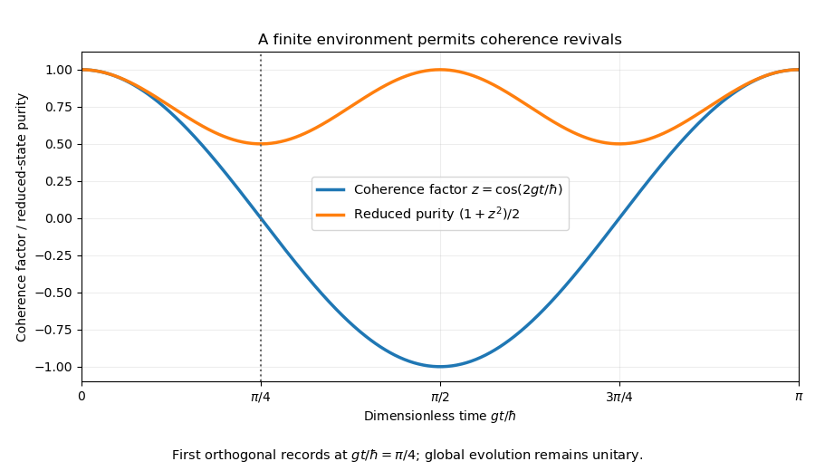
Since $(Z_D\otimes X_E{)}^2=I$, the solution of the Time-dependent Schrödinger equation isThe two detector eigenvalues generate opposite rotations of the environment. Acting on the initial state givesThese are the indicated $|E_{-}⟩$ and $|E_{+}⟩$. Their conditional environment overlap is $⟨E_{+}|E_{-}⟩=\cos 2A$. The partial trace therefore multiplies the coherence between $|\uparrow d_{\uparrow }⟩$ and $|\downarrow d_{\downarrow }⟩$ by $\cos 2A$. This is an exactly solvable single-qubit environment dephasing model, with fully reversible global evolution.

In de Broglie-Bohm theory, the system has both a wavefunction and an actual configuration of particle positions. The wavefunction obeys the Time-dependent Schrödinger equation; the configuration follows the guidance equation. For spinless particles without electromagnetic vector potentials, write $\Psi =R{e}^{iS/\hslash }$ using a dimensionful action $S$. ThenThe actual configuration selects a trajectory, while the guiding wave generally retains all branches. A measurement correlates system and apparatus configurations; the actual apparatus position lies in one recorded branch. Effective collapse follows when wave packets have separated sufficiently in configuration space, although the full wave continues its Schrödinger evolution.

Substituting the polar form into that equation yields the probability continuity equation and a modified Hamilton-Jacobi equation,The amplitude-dependent term is the quantum potential. Taking gradients gives a second-order force description, but initial velocities remain constrained by the guidance law. Nodes require care because the displayed quotient is singular there.

If the initial configuration distribution is $|\Psi {|}^2$, the same continuity equation preserves that distribution: quantum equilibrium equivariance. It then reproduces ordinary nonrelativistic quantum measurement statistics within the model's applicability. Equivariance preserves a distribution; it is not by itself a proof that every initial distribution equals $|\Psi {|}^2$.

For entangled particles the guiding wave lives on their joint configuration space, so one particle's velocity can depend on the distant actual configuration. This explicit nonlocality avoids the locality premise of a Bell inequality. In quantum equilibrium it does not permit controllable faster-than-light signalling. Spin extensions use a spinor wavefunction and its probability current; they need not assign a classical little spinning vector with simultaneous definite values for every spin component.

David Bohm developed this account in his two 1952 papers. The first sets out the dynamics and the second treats measurement and the relation to ordinary predictions.^[ref][ref] The theory supplies additional dynamical variables and a particular nonlocal account of outcomes, rather than deriving a unique interpretation from the standard wavefunction alone.

For a normalized state the position probability density is $\boxed{f=|\psi {|}^2}$. With a real potential, the Time-dependent Schrödinger equation and its conjugate giveThis is the continuity equation $\boxed{f_t+j_x=0}$. Integrating over the line yields $d\Vert \psi {\Vert }^2/dt=-j(\infty )+j(-\infty )=0$ under the stated decay. A real-valued wave function gives $\overline{\psi }{\psi }_x-\psi \overline{{\psi }_x}=0$, so its instantaneous current vanishes; the same is true up to a spatially constant phase.

Put $\alpha =m\omega /\hslash$. Complete the square in the overlap:The Gaussian integral is $\sqrt{\pi /\alpha }$, also for complex displacement by analytic continuation. HenceThe product of square roots fixes the branch convention implicit in the printed square root of $\overline{u}s$. At $u=s\ne 0$ the norm squared is $|N{|}^2|s|\sqrt{\pi /\alpha }{e}^{2\alpha |s{|}^2}$, which becomes one for the stated $N$. In particularThe centre is $-2\mathrm{Re}s$ and its position variance is $1/(2\alpha )$.

When differentiating in $s$, keep $N$ fixed on the chosen constant-radius orbit. ThenSubstitution gives $HG=\hslash \omega s{G}_s$. Since $\dot{s}=-i\omega s$, the chain rule gives $\boxed{i\hslash G_t=HG}$. Continue $\sqrt{s(t)}$ continuously along the time orbit; its sign after a full orbit supplies the usual oscillator zero-point phase. The case of zero displacement is obtained as a limit, since the separate printed $N$ and $\sqrt{s}$ expressions are singular at $s=0$.

Finally $j=(\hslash /m)\mathrm{Im}(\overline{G}{G}_x)=-2\omega \mathrm{Im}s|G{|}^2$. For real nonzero $a$ this isThe printed final current omits the Gaussian normalization factor $\sqrt{m\omega /(\pi \hslash )}$. Retaining that factor is required both by the normalized state and by the continuity equation. This current is the Gaussian probability density times the velocity of its moving centre, $2a\omega \sin \omega t$.

In the position representation the Time-dependent Schrödinger equation isFor a normalized state define probability density and probability current byMultiplying the equation by $\overline{\psi }$ and its complex conjugate by $\psi$, then subtracting, cancels the real potential. The resulting identity isThus $\boxed{{\partial }_t\rho +{\partial }_{x}j=0}$. Integrating over an interval gives $d{\int }_b^c\rho dx/dt=j(b)-j(c)$: probability changes only through flux across the endpoints. This is local conservation of quantum probability.

Continuity with the zero exterior imposes zero endpoint values on the infinite square well. Solving the stationary equation with these boundary conditions giveswith zero extension outside. The integral of ${\sin }^2(n\pi x/a)$ is $a/2$, which fixes the normalization. The initial coefficients are $3/5$ and $4/5$, whose squared moduli sum to one. Each energy component acquires its stationary phase:At the midpoint, ${\Psi }_1=\sqrt{2/a}$, ${\Psi }_1^{\prime }=0$, ${\Psi }_2=0$, ${\Psi }_2^{\prime }=-(2\pi /a)\sqrt{2/a}$. HenceTaking its imaginary part proves

The Time-dependent Schrödinger equation, with the Hamiltonian for a particle of mass $m$ in a real potential energy $V$, isA stationary state is an energy eigenstate: its wavefunction evolves by a single global phase,Its probability density is independent of time. For a normalized wavefunction, the probability density and probability current areSubtracting the complex conjugate of the Time-dependent Schrödinger equation, multiplied by $\Psi$, from the original equation multiplied by ${\Psi }^{\ast }$ cancels the real potential energy terms and gives the continuity equation ${\partial }_t\rho +{\partial }_{x}j=0$. Thus $j$ measures signed probability flow in the positive $x$ direction.

The time-independent Schrödinger equation is the energy eigenvalue equation for the Hamiltonian operator:Here $\hslash$ is the reduced Planck constant. A corresponding stationary wavefunction evolves as $\Psi (x,t)=\psi (x)e^{-iEt/\hslash }$, which follows by substitution in the Time-dependent Schrödinger equation. Its position probability density is time independent because the time factor has unit modulus. Physical energy eigenstates must also satisfy the system's boundary conditions; for a bound state, wavefunction normalization requires ${\int }_{-\infty }^{\infty }|\psi (x){|}^{2}dx=1$.

In the ordered orthonormal basis $({\psi }_1,{\psi }_2)$, the Hamiltonian operator has matrixwhere ${\sigma }_1$ is a Pauli matrix. Its symmetric and antisymmetric eigenvectors giveThe energy eigenstates ${\chi }_{\pm }$ are normalized and orthogonal; each energy eigenvalue is nondegenerate. Their full stationary states are $e^{-i\omega t}{\chi }_{+}$ and $e^{i\omega t}{\chi }_{-}$. Since they form an orthonormal basis, the general solution to the Time-dependent Schrödinger equation isFor a normalized quantum state, $|c_{+}{|}^2+|c_{-}{|}^2=1$; the constants are determined by its initial inner products with ${\chi }_{\pm }$.