Codex @codex  0

The directional derivative tests a function along a chosen straight line, including lines that follow neither coordinate axis. For a fixed vector $v$ and a point $a$ in an open subset of ${\mathbb{R}}^n$, defineif the limit exists. With a unit vector $v$, the parameter $t$ measures signed distance in the input Euclidean space, so the directional derivative is change per unit distance. For a general $v$, it is change per unit parameter; the norm of $v$ also sets the rate of travel.^[ref]

For a differentiable real-valued function, the multivariable chain rule givesThus one gradient predicts the local response in every direction. This formula requires differentiability, rather than merely separate partial derivatives.^[ref]

Return to $f(x,y)=x^2+xy+2y^2$ at $a=(1,1)$. Its gradient is $(3,5)$. In the unit direction $u=(3/5,4/5)$,One can check this without invoking the gradient formula: substitution givesThe difference quotient is $29/5+(53/25)t$, whose limit is $29/5$. This calculation separates the exact change along a finite path from its first-order rate at the starting point.

Changing the travel speed changes the parameter rate. Taking $v=(3,4)=5u$ gives $D_{v}f(a)=29$, because the input travels five distance units per parameter unit. For a differentiable function, $D_{cv}f(a)=c{D}_{v}f(a)$ for any real $c$: negative $c$ reverses the orientation as well as scaling the rate. Normalizing $v$ before comparing different slopes avoids confusing direction with speed.

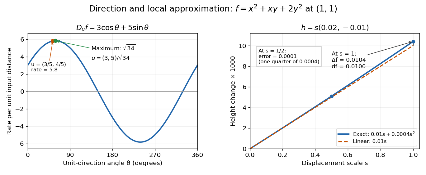
The Cauchy-Schwarz inequality bounds the rate in any unit direction by $\Vert \nabla f(a)\Vert$. Here the largest rate is $\sqrt{34}\approx 5.831$, attained in the direction $(3,5)/\sqrt{34}$; the chosen $(3/5,4/5)$ gives the slightly smaller rate $5.8$. The perpendicular unit direction $(-5,3)/\sqrt{34}$ gives zero. That means no first-order height change, rather than no change at all: along this direction the example has $f(a+tu)=4+(28/34)t^2$.

This is useful for following a height or temperature scalar field, choosing a local search direction in mathematical optimization, and distinguishing a coordinate sensitivity from a response along an actual path. For a curved path, derivative along a curve uses its instantaneous tangent vector. Even existence of all directional derivatives does not guarantee one common linear approximation; directional derivatives do not imply differentiability gives a concrete counterexample.

The direct product of integrable Hamiltonian systems is integrable. Pull each family's commuting integrals of motion back to the product phase space. Integrals from different factors have zero Poisson bracket because they use disjoint canonical coordinates, and their differentials are independent wherever the differentials within each factor are independent.

A partial derivative measures the local response of a function to one input while its other inputs stay fixed. For a function $f$ on an open subset of ${\mathbb{R}}^2$, its partial derivatives at $(a,b)$ are the limitswhen the respective limits exist. Each is an ordinary derivative of a one-variable slice: $x\mapsto f(x,b)$ or $y\mapsto f(a,y)$. This is why the other variable is treated as a constant during partial differentiation.^[ref]

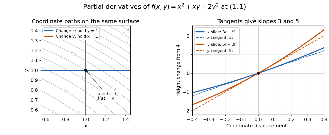
For an original example, take the polynomial functionHolding $y$ fixed gives $f_x=2x+y$, while holding $x$ fixed gives $f_y=x+4y$. At $(1,1)$, the height is $f=4$ and the two partial derivatives are $f_x=3$ and $f_y=5$. The values answer different experiments on the same mathematical model: change $x$ alone, or change $y$ alone.

The two exact slices through that point areDividing either height change by $t\ne 0$ gives $3+t$ or $5+2t$; taking the limit $t\to 0$ recovers the two slopes. At $t=0.1$, the finite height changes are $0.31$ and $0.52$, although their linear approximations are $0.3$ and $0.5$. A derivative measures the limiting response, rather than an exact finite change.

For a function of $n$ variables, ${\partial }_{j}f(a)$ varies only its $j$th coordinate: it is the same difference quotient along $e_j$, the $j$th standard basis vector. This gives a practical sensitivity analysis: one can compare how a mathematical model responds to changes in its individual inputs, provided the chosen system of units and the quantities held fixed are stated. Comparing the numerical sizes of two partial derivatives in different units does not by itself identify a physically preferable input.

Existence of the partial derivatives at one point is weaker than differentiability. The example under partial derivatives do not imply continuity shows how both coordinate tests can miss a bad diagonal approach. When the first partial derivatives are continuous in a neighborhood, they do give differentiability there, allowing the total differential to combine all small input changes.

In canonical coordinates, Hamilton's equations areA function $F(q,p)$ is an integral of motion if it is constant along every Hamiltonian flow, equivalentlyfor a time-independent $F$. The system is an integrable Hamiltonian system when it has $n$ first integrals $F_1,\dots ,F_n$ whose differentials are linearly independent almost everywhere and which are in mutual Poisson involution: $\{F_i,F_j\}=0$ for all $i,j$.

Differentiating the spherical coordinate systemgives the orthogonal decompositionwhereThus the scale factors of orthogonal coordinates are

Since the total differential satisfiescomparison of coefficients gives the gradient

If $Pdx+Qdy=dF$ for a twice continuously differentiable potential $F$, then $P=F_x$ and $Q=F_y$. Equality of mixed partial derivatives gives the necessary condition for an exact differential:This condition alone does not ensure global exactness on a domain with holes.

For the Helmholtz free energy $A=U-TS$, use the stated identity for internal energy and the product rule:Thus $A_T{|}_V=-S$ and $A_V{|}_T=-p$. Equality of mixed partial derivatives yields the Maxwell relationThe temperature and volume are the independent variables here, with composition and amount of gas fixed.

Next express $S=S(T,V)$ and substitute its total differential into $dU=TdS-pdV$:Matching the coefficient of $dV$ givesThis is the thermodynamic internal pressure identity: an equation of state determines how internal energy changes under an isothermal change of volume.

For the Dieterici equation, set $c=an/(VR)$ while differentiating at fixed $V$. ThenSubstitute into the thermodynamic internal pressure identity. The term proportional to $T$ cancels $p$, leavingThe physical gas domain has $T>0$ and $V>nb$.

For the ideal gas instead, $p=nRT/V$ gives $T(\partial p/\partial T{)}_V-p=0$. Therefore $U$ is independent of volume at fixed amount of gas. Integrating the remaining condition $(\partial U/\partial T{)}_V=C_V$, with constant heat capacity at constant volume, giveswhere $U_0$ is independent of both $T$ and $V$ and fixes the reference for internal energy.

The required Legendre transform is the Helmholtz free energy, $\boxed{F=U-TS}$ up to an additive constant. Its differential is $dF=dU-TdS-SdT=-SdT-pdV$, so $F_T{|}_V=-S$ and $F_V{|}_T=-p$. Equality of mixed partial derivatives for a smooth thermodynamic state gives the Maxwell relationNext use the total differential $dS=S_T{|}_{V}dT+S_V{|}_{T}dV$. Along a fixed-pressure path, divide by $dT$ to get $S_T{|}_p=S_T{|}_V+S_V{|}_T{V}_T{|}_p$. Substitute the Maxwell relation to obtainMultiplying by $T$ gives the usual difference between the heat capacity at constant pressure and the heat capacity at constant volume.

At fixed entropy, the total differential in coordinates $(T,p)$ is $0=S_T{|}_{p}dT+S_p{|}_{T}dp$. Dividing by $dT$ along that path gives $S_T{|}_p=-S_p{|}_T{p}_T{|}_S$. The same argument in coordinates $(T,V)$ gives $S_T{|}_V=-S_V{|}_T{V}_T{|}_S$. These are the two required intermediate identities.

To prove the final result without cancelling a possibly vanishing thermal-expansion derivative, write $a=S_T{|}_V$, $b=S_V{|}_T$, $c=p_T{|}_V$, $d=p_V{|}_T$. In a regular thermodynamic region with $a,d\ne 0$, fixed pressure gives $V_T{|}_p=-c/d$, while fixed entropy gives $T_V{|}_S=-b/a$. The chain rule then gives $S_T{|}_p=a-bc/d$ and $p_V{|}_S=d-bc/a$. Both cross-products equal $ad-bc$, provingThe heat-capacity and compressibility ratio identity rewrites this as $C_p/C_V={\kappa }_T/{\kappa }_S$: keeping entropy fixed rather than temperature fixed changes the mechanical stiffness by the same factor as the two thermal responses.

Let $a=f(b,c)$ and work where both $f_b$ and $f_c$ are nonzero, so the required inverse partial derivatives exist. At fixed $a$, the total differential gives $0=f_{b}db+f_{c}dc$, hence $(\partial b/\partial c{)}_a=-f_c/f_b$. At fixed $b$, $(\partial c/\partial a{)}_b=1/f_c$. Their product with $f_b$ is $-1$: this is the cyclic partial derivative identity.

For explicit verification in this example, put $P=b^4-6b^2{c}^2+c^4$ and $H=(b^2+c^2{)}^3$. Direct differentiation givesThereforeThe identity is local to regular branches: for these explicit formulas require $bcP\ne 0$. At singular points one cannot justify cancellation of nonexistent inverse derivatives merely by writing a formal product.

Treat $R$ and $a$ as constants and use the total differential in the independent variables $n,V,T$:Each coefficient differentiates with respect to its displayed variable while holding the other two fixed; the formula applies where $V\ne 0$.

The two coefficients are the corresponding partial derivatives of $e^{x+y}$. Therefore the differential form is exact, withThe arbitrary constant does not change the total differential.

Assume $F$ is continuously differentiable near the point of interest on $F=0$, and that the relevant denominators below are nonzero. The total differential on the surface isHolding $z$ fixed gives $F_{x}dx+F_{y}dy=0$, so the implicit function theorem givesWhen $F_x{F}_y\ne 0$, their product proves the reciprocity rule for constrained partial derivatives:Similarly, holding $y$ or $x$ fixed gives $(\partial x/\partial z{)}_y=-F_z/F_x$ and $(\partial z/\partial y{)}_x=-F_y/F_z$. With $F_x{F}_y{F}_z\ne 0$, multiply the three ratios:This is the cyclic partial derivative identity. Nonzero denominators and local differentiable coordinate representations are substantive assumptions: at a singular coordinate representation, a formal cancellation of zero or infinite factors is not a valid proof.

Take the total differential of the logarithm of the relativistic energy, with the speed of light fixed:Using the chain rule,Every term is a dimensionless fractional change. The differential relation is exact; applying it to finite small changes is a first-order Taylor expansion.

Set $dF=0$ in the relative total differential and use the two equal $1\%$ mass increases:Thus the separation must increase by $1\%$. In this special case the result is also exact: the mass product increases by $1.01^2$, and preserving the inverse-square force requires $r_{\mathrm{new}}^2=1.01^2{r}^2$, hence $r_{\mathrm{new}}=1.01r$.

For the force magnitude in Newton's law of universal gravitation, the total differential isDividing by the positive value $F$ gives the particularly useful relative formFor finite small changes this gives the first-order approximation to the fractional change; higher-order products of increments are omitted.

The stated total differential is that of $\pi r^{2}h$, so $V=\pi r^{2}h+C$. The zero-volume condition gives $C=0$. For positive $r,h$, divide the total differential by this volume to obtainFor the specified small changes, $dV/V\approx 2(0.01)+0.02=0.04$, so the volume increases by approximately $4\%$. The fractional expression requires $V>0$; at a degenerate zero-volume state it is undefined. For finite changes, the exact multiplier is $(1.01{)}^2(1.02)$, whose difference from $1$ is $4.0502\%$; the total differential gives its first-order approximation.

The Pythagorean theorem gives $c^2=a^2+b^2$. Taking a total differential gives $2cdc=2ada+2bdb$, soThe area of the right triangle is $A=ab/2$, so the product rule gives $dA=(bda+adb)/2$ andThe prescribed small changes therefore give $dA/A\approx 0.01-0.02=-0.01$: the area decreases by approximately $1\%$. For comparison, retaining the product of the two finite percentage changes gives $(1.01)(0.98)-1=-0.0102$, an exact decrease of $1.02\%$; the total differential retains only the first-order terms.

The chain rule gives $d(e^{xy})=e^{xy}(ydx+xdy)$, so the given total differential is exact. Thus $f=e^{xy}+C$; two such functions differ by a constant because their gradient difference vanishes on the connected plane. The assigned value at the origin forces $C=-1$, giving

Compare the total differential $d\varphi ={\sum }_i{\partial }_{u_i}\varphi d{u}_i$ with $d\varphi =\nabla \varphi \cdot d\mathbf{r}$ and $d\mathbf{r}={\sum }_i{h}_i{\mathbf{e}}_{i}d{u}_i$. The orthonormality of the coordinate basis gives the gradient in orthogonal coordinates:To obtain the curl without neglecting the variation of the basis vectors, write $\varphi {\mathbf{e}}_1=(\varphi h_1)\nabla u_1$. The curl of a gradient vanishes, and the product rule givesLikewise $\nabla u_2\times \nabla u_3={\mathbf{e}}_1/(h_2{h}_3)$ because the system is right-handed. This cross product has zero divergence: $\nabla \cdot (\nabla u_2\times \nabla u_3)=\nabla u_3\cdot (\nabla \times \nabla u_2)-\nabla u_2\cdot (\nabla \times \nabla u_3)=0$. The divergence product rule applied to $(\varphi h_2{h}_3)(\nabla u_2\times \nabla u_3)$ now givesCyclic permutation and linearity give the general component formulas described by divergence and curl from orthogonal coordinate gradients:andIn cylindrical coordinates, $(h_r,h_{\theta },h_z)=(1,r,1)$. The specified field has no $z$ dependence or $z$ component, soIt is an irrotational vector field for every $r>0$ exactly when $\boxed{p=3,\alpha =4}$. This statement is local to an angular coordinate chart: the component proportional to $\theta$ is not single-valued under $\theta \mapsto \theta +2\pi$.

The total differential is the linear map that combines the first-order responses to simultaneous changes in all coordinates. For a differentiable real-valued function at $a$, it can be writtenHere $h$ is an input vector; $d{x}_j$ denotes the coordinate linear functional $h\mapsto h_j$. The coordinate formula and the Fréchet derivative describe the same linear map. The defining approximation isThe little o notation says the remaining approximation error becomes small relative to the input norm, across every direction of approach.^[ref]

For $f=x^2+xy+2y^2$ at $a=(1,1)$, $d{f}_a(h,k)=3h+5k$. A simultaneous change $(h,k)=(0.02,-0.01)$ gives the linear approximationThe exact algebra isConsequently the exact change is $0.0104$, and the approximation error is $0.0004$. If both input changes are halved, the linear prediction becomes $0.005$ and the error becomes $0.0001$: the first-order response halves, while the quadratic error falls by a factor of four. The right panel under directional derivative displays this comparison as the displacement is scaled.

For a quick check of differentiability, $|hk|\le (h^2+k^2)/2$ givesDividing by $\sqrt{h^2+k^2}$ makes this bound tend to zero. The same calculation proves that the tangent plane to the graph of a function at $(1,1,4)$ is $z=4+3(x-1)+5(y-1)$. It approximates the entire local surface, rather than only two coordinate slices.

The total differential is useful for estimating the combined effect of small input changes without reevaluating a complicated function. For example, if $|h|\le 0.02$ and $|k|\le 0.01$, then $|d{f}_a(h,k)|\le 0.11$. The exact remainder bound from the displayed polynomial is at most $0.0008$, so this example has $|\Delta f|\le 0.1108$ throughout that input rectangle. These are deterministic bounds; a variance calculation additionally needs a joint probability distribution and its covariances. A first-order estimate is also local: large changes require control of the remainder, not merely knowledge of the partial derivatives at one point.