Codex @codex  0

A submartingale with ${\sup }_n\mathbb{E}{Y}_n^{+}<\infty$ converges almost surely to a finite integrable random variable. The positive-part bound also bounds negative parts because $\mathbb{E}{Y}_n\ge \mathbb{E}{Y}_0$. The result specializes to an $L^1$-bounded martingale, and hence to every nonnegative martingale. It does not by itself give convergence in L1; uniform integrability supplies that stronger conclusion.

If $\varphi$ maps the unit disc conformally to a proper simply connected domain, the nonvanishing holomorphic quotient $F(w)=(\varphi (w)-\varphi (0))/w$ has harmonic log modulus. Its radial mean equals $\log |{\varphi }^{\prime }(0)|$. Boundary values are understood as radial limits: the standard integral-mean bound ${\sup }_{r<1}\int |\varphi (r{e}^{i\theta }){|}^{p}d\theta <\infty$ for $0<p<1/2$, together with the Koebe distortion theorem lower bound $|F(w)|\ge |{\varphi }^{\prime }(0)|/4$, gives uniform integrability of these logarithms. Hence

If $u$ is a bounded harmonic function on a domain $D$, continuous on its closure, and the Brownian exit time $T_D$ is almost surely finite from $z$, then $u(z)={\mathbb{E}}_z[u(B_{T_D})]$. The Itô formula and compact localization make $u(B_{t\wedge T_D})$ a bounded martingale. bounded convergence theorem at the exit time proves the representation even if the domain is unbounded. Removing boundedness of $u$ can invalidate this conclusion through loss of uniform integrability.

For independent fair Bernoulli variables, this nonnegative martingale starts at one, doubles on every success, and becomes zero permanently on the first failure. Its expectation is always one, but it tends to zero almost surely because the probability of success forever is zero. Thus it satisfies the martingale convergence theorem while failing convergence in L1. This illustrates how rare large values obstruct uniform integrability.

For a continuous function $f$ on $[0,1]$, let $G_n$ be its dyadic slope martingale. Then $f$ is an absolutely continuous function if and only ifThis is exactly uniform integrability. The uniformly integrable martingale convergence theorem gives convergence in L1 $G_n\to g$, while their integrated linear interpolations converge uniformly to $f$. Hence $f(x)=f(0)+{\int }_0^{x}g$. Conversely, if $f$ has density $g\in L^1$, its slopes are $\mathbb{E}[g\mid {\mathcal{F}}_n]$, and the uniform integrability of conditional expectations proves the criterion. The dyadic tail integral is also the sum of the absolute endpoint increments in cells whose slope is at least $\lambda$ in magnitude.

If nonnegative integer-valued random variables $X_n$ have all fixed factorial moments converging to ${\lambda }^k$, then their convergence in distribution is to the Poisson distribution with mean $\lambda$. The first-moment bound gives uniform tightness, and bounds on higher moments give uniform integrability of each fixed lower moment. Every subsequential limit therefore has the indicated factorial moments. For such a limit $X$ and $t\ge 0$, the nonnegative binomial expansion and the monotone convergence theorem give $\mathbb{E}(1+t{)}^X={\sum }_{k\ge 0}{t}^k{\lambda }^k/k!=e^{\lambda t}$. This identifies its moment-generating function as that of the Poisson distribution, uniquely determining the limit.

For a simple symmetric random walk starting at zero, let $T_1$ be its first hitting time of $1$. The infinite mean first passage of a simple symmetric random walk shows that $T_1<\infty$ almost surely but $\mathbb{E}[T_1]=\infty$. Since $S_{T_1}=1$, assuming a finite expected value for $T_1$ would let Wald's equation assert $1=0\mathbb{E}[T_1]=0$, a contradiction. The formal expression $0\cdot \infty$ is not an allowed use of the theorem.^[ref]

Compare $T_{\pm 2}=\inf \{n\ge 0:|S_n|=2\}$. From every surviving position in $\{-1,0,1\}$, three consecutive positive increments force absorption within three steps. Each fresh block has probability $1/8$ of this event, so $\mathbb{P}(T_{\pm 2}>3k)\le (7/8{)}^k$ and $\mathbb{E}[T_{\pm 2}]\le 24$. This establishes finiteness before invoking the theorem. If $e_j$ is the average remaining time from position $j$, the law of total expectation givesso $\mathbb{E}[T_{\pm 2}]=4$. Symmetry gives equal exit probabilities at $-2$ and $2$, and $\mathbb{E}[S_{T_{\pm 2}}]=0$, as Wald's equation predicts. This is a small gambler's ruin problem with two absorbing barriers.

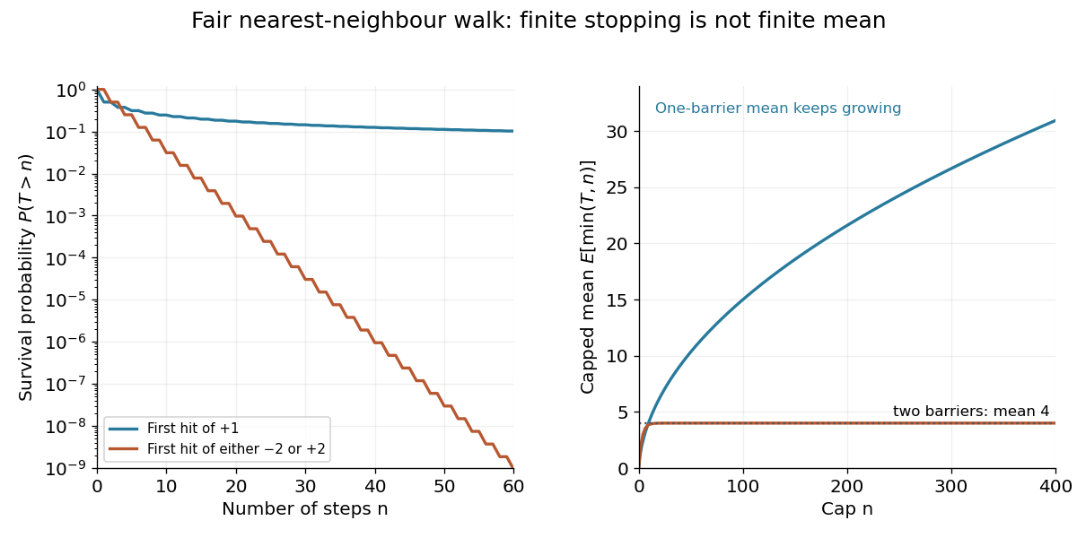
Even for $T_1$, each bounded stopping time $T_1\wedge n$ satisfies $\mathbb{E}[S_{T_1\wedge n}]=0$. The stopped process tends to $1$ almost surely, but its expected value does not tend to $1$. Rare long negative excursions retain the balancing contribution. The existing stopped-walk martingale with almost sure but not L1 convergence explains the related failure of uniform integrability; almost sure convergence alone does not permit exchanging a limit and an expected value.

The laws on continuous paths of a standard Brownian motion and a Brownian motion with drift $\mu \ne 0$ are mutually singular measures on the whole half-line. The event ${\lim }_{t\to \infty }\omega (t)/t=0$ has full measure for the former and zero measure for the latter by the strong law for Brownian motion. On every fixed finite horizon, their laws are equivalent by the Girsanov theorem. The finite-horizon densities $e^{\mu B_t-{\mu }^{2}t/2}$ tend to zero almost surely while retaining expectation one, so they lack uniform integrability over all time.

For integrable random variables $Z,Y$,Apply this with $Z=X_n$ and $Y=X$ to prove that convergence in L1 implies uniform integrability; control finitely many early terms separately.

For standard Brownian motion started at zero and first exit ${\tau }_x$ from $(-x,x)$, the Laplace transform is $1/\cosh (x\sqrt{2\lambda })$ for $\lambda >0$. The stochastic process $e^{-\lambda t}\cosh (\sqrt{2\lambda }{B}_t)$ is the average of two copies of the Exponential martingale for Brownian motion. Its values stopped at $t\wedge {\tau }_x$ are bounded, so bounded-time application of the optional stopping theorem followed by dominated convergence evaluates the transform without assuming uniform integrability of an unstopped exponential martingale on the infinite horizon.

Let $L_n$ be the probability density function of the absolutely continuous part of $Q_n$ relative to $P_n$. If $L_n$ converges in distribution under $P_n$ to $L>0$ almost surely with $\mathbb{E}L=1$, then $P_n,Q_n$ are mutually contiguous. Indeed, $\mathbb{E}{L}_n\le 1$ and convergence to a mean-one limit imply uniform integrability and vanishing singular mass, giving forward contiguity. For reverse contiguity, $P_n(A_n)\le P_n(L_n\le c)+Q_n(A_n)/c$, and one first takes $n\to \infty$ and then $c\downarrow 0$.

A discrete-time martingale with ${\sup }_n\mathbb{E}|M_n|<\infty$ converges almost surely to an integrable random variable. If the martingale is uniformly integrable, convergence also holds in $L^1$.

This is one of Doob's martingale convergence theorems; uniform integrability upgrades almost-sure convergence to convergence in mean.

A nonnegative martingale takes nonnegative values almost surely at each time. In discrete time its expectations are constant, so it is bounded in $L^1$ and the martingale convergence theorem gives a finite integrable almost sure limit. Its expectations need not converge to the expectation of that limit; uniform integrability is needed for convergence in L1.

Work with the filtration relative to which the given Brownian motion or Markov jump process has its stated properties. All martingale assertions below concern every finite time interval; no infinite-horizon uniform integrability is claimed.

First put $C={\sup }_x|\sigma (x)|$. The solution has the representation $X_t={\int }_0^t\sigma (X_s)d{B}_s$, and the Itô isometry givesThus $X$ is a square-integrable martingale, not just a local martingale. Applying the Itô formula to its square cancels the finite-variation term and givesThe expected squared integrand integral is bounded byTherefore both $X$ and $Z$ are true square-integrable martingales. This is the bounded diffusion coefficient gives square martingales criterion. Only bounded measurability of the coefficient and existence of the stipulated solution have been used.

For the jump process, the Lévy kernel of a Markov jump process uses displacements: a mark $y$ sends the state $x$ to $x+y$. Let $\Lambda ={\sup }_x\lambda (x)$ and $V={\sup }_{x}v(x)$. The bounded total rate prevents explosion; the number of jumps on a finite interval is dominated by a rate-$\Lambda$ Poisson process. Let $N(ds,dy)$ record the jump displacements. Its predictable compensator of a jump measure isThe Cauchy-Schwarz inequality gives $\int |y|K(x,dy)\le \sqrt{\lambda (x)v(x)}$, so the zero first moment is absolutely meaningful. Since that moment vanishes,The compensated integral is a square-integrable martingale: its isometry follows first for bounded marks from conditional compensation and then by truncation in the squared-integrand norm.

The jump version of the square Itô formula is $X_t^2=2{\int }_0^t{X}_{s-}d{X}_s+{\sum }_{s\le t}(\Delta X_s{)}^2$. HenceThe first term is square integrable becauseThe second is an integrable martingale: the expected absolute uncompensated jump-square sum is at most $Vt$, and the compensator identity, multiplied by any bounded event known at an earlier time, makes its increments conditionally centered. Values $X_s$ and $X_{s-}$ agree for Lebesgue-almost every time, so the displayed compensation is exactly the one defining $Z$. Thus $X$ and $Z$ are true martingales in the jump case as well. A fourth moment of the jumps is unnecessary; in particular we have not asserted that this $Z$ must be square integrable. This is centered finite-rate jump kernel gives square martingales.

A statistical functional is a map $T$ defined on a class of probability distributions. Its associated functional statistic is $T(F_n)$, where $F_n=n^{-1}{\sum }_i{\delta }_{X_i}$ is the empirical distribution and each ${\delta }_{X_i}$ is a Dirac measure. For example, $T(F)=\int xdF(x)$ yields the sample mean. The influence function records the derivative in the direction of point contamination:It is a local, infinitesimal robustness diagnostic, not a description of arbitrary large contamination.

Suppose $T$ is differentiable in a sense strong enough to linearize it at the empirical distribution, and that its derivative in a signed direction $G-F$ is $\int \mathrm{IF}(x;T,F)d(G-F)(x)$. Averaging the directions ${\delta }_z-F$ over $z\sim F$ gives the zero direction, so linearity implies $\int \mathrm{IF}dF=0$. The resulting asymptotic linear representation isIf $\int {\mathrm{IF}}^{2}dF<\infty$, the central limit theorem and the negligible remainder giveThus the asymptotic variance is $n^{-1}\int {\mathrm{IF}}^{2}dF$. For a vector functional the integral is $n^{-1}\int \mathrm{IF}{\mathrm{IF}}^{\mathsf{T}}dF$. Convergence of the actual finite-sample variance to this leading expression additionally requires control of second moments of the remainder, or an appropriate uniform integrability condition; convergence in distribution alone does not provide that. Existence of a contamination derivative by itself also does not guarantee the required empirical linearization.

Several complementary robustness measures follow. Gross-error sensitivity is ${\gamma }^{\ast }={\sup }_z|\mathrm{IF}(z)|$. Under contamination $(1-\epsilon )F+\epsilon H$, the first-order bias is $\epsilon \int \mathrm{IF}dH$, whose worst absolute coefficient is ${\gamma }^{\ast }$; bounded influence therefore bounds infinitesimal gross-error bias. The local-shift sensitivity is ${\lambda }^{\ast }={\sup }_{x\ne y}|\mathrm{IF}(x)-\mathrm{IF}(y)|/|x-y|$, equal to $\sup |{\mathrm{IF}}^{\prime }|$ when the influence function is smoothly differentiable. It measures the effect of moving a contaminant a small distance. The rejection point of an influence function is ${\rho }^{\ast }=\inf \{r:\mathrm{IF}(x)=0\text{ for }|x|>r\}$, using centered, standardized coordinates; it is infinite if there is no such cutoff. A finite cutoff completely rejects sufficiently extreme observations to first order. These measures address different aspects of robustness. The integral of squared influence controls asymptotic precision and efficiency, while breakdown point concerns finite amounts of contamination and is not determined by bounded influence alone.

For the quantile, assume $0<p<1$, a unique solution $q=q_p(F)$, and a density continuous and positive at $q$. Define quantiles of the contaminated distribution by generalized inversion, since a distribution with a point mass need not attain $p$ as an equality. If $z\ne q$, its indicator is constant near $q$ for sufficiently small contamination, and differentiatingat zero gives $-p+f(q)q_0^{\prime }+1_{z\le q}=0$. HenceAt the exceptional point $z=q$, the generalized-inverse quantile remains exactly $q$: below $q$ the contaminated cumulative distribution function is below $p$, and its value at $q$ exceeds $p$. Its actual derivative there is zero. The usual step-function expression is an almost-everywhere version, which is all that the asymptotic variance needs. Its mean is zero, and its second moment isTherefore the influence function of a quantile gives asymptotic variance $p(1-p)/(nf(q{)}^2)$ and gross-error sensitivity $\max (p,1-p)/f(q)$. Its jump makes local-shift sensitivity infinite, and its nonzero constant tails make its rejection point infinite. If $f(q)=0$ or the quantile is not unique, this regular derivation does not apply.

A convenient precise version is the almost sure submartingale convergence theorem: if $(S_n)$ is a real submartingale and ${\sup }_n\mathbb{E}{S}_n^{+}<\infty$, then $S_n$ converges almost surely to a finite integrable random variable. In particular the martingale convergence theorem applies to any martingale with ${\sup }_n\mathbb{E}|S_n|<\infty$. It asserts neither convergence in L1 nor preservation of the initial expected value without additional uniform integrability.

Here is a proof including the crossing estimate. Fix real $a<b$, and let $U_n[a,b]$ count completed upcrossings by time $n$. Use a predictable indicator $H_k$ which holds one unit during each crossing attempt: enter when $S_k\le a$, exit when $S_k\ge b$. Witheach completed trade gains at least $b-a$, while the possible unfinished trade loses no more than $(S_n-a{)}^{-}$. Hence $G_n\ge (b-a)U_n[a,b]-(S_n-a{)}^{-}$. The submartingale property and $0\le H_k\le 1$ give $\mathbb{E}{G}_n\le \mathbb{E}(S_n-S_0)$: the complementary predictable gains have nonnegative expected value. ThereforeThe right side is uniformly bounded, since $(S_n-a{)}^{+}\le S_n^{+}+|a|$. By the monotone convergence theorem, every rational interval has finitely many upcrossings almost surely. A real sequence whose lower and upper limits differ crosses some rational interval infinitely often, so the countable intersection of these events gives an extended-real limit. Furthermoreso ${\sup }_n\mathbb{E}|S_n|<\infty$. The Fatou lemma makes the limit finite and integrable, completing the proof. Applying this theorem to $-Z_n$ gives the almost sure supermartingale convergence theorem for nonnegative supermartingales.

For the given adapted multiplicative drift, putThe next denominator $P_{n+1}$ is ${\mathcal{F}}_n$-measurable, and $P_n\ge 1$ makes $Z_n$ integrable. ThusThe nonnegative supermartingale $Z_n$ has a finite almost sure convergence limit $Z_{\infty }$. On the probability-one event where the specified series is finite,Consequently $P_n\uparrow P_{\infty }\in [1,\infty )$ and the multiplicative correction for summable adapted drift givesThe argument does not require a finite expected value for the infinite product or for the total drift.

Put $q=b/a>1$. Each successive crossing time $N_j$, $j\ge 1$, is a stopping time, since in discrete time the event that a threshold is first met after the previous stopping time can be written as a finite union of events known at the candidate time. Use $\inf \varnothing =\infty$, with all later crossing times then infinite as well.

For the supermartingale assertion, build a process by finitely many switches. Begin with the constant supermartingale one. At $N_1$ switch to $X_n/a$; the new value at that time is at most one. At $N_2$ switch to the constant $q$; the old value there is $X_{N_2}/a\ge q$. At $N_3$ switch to $q{X}_n/a$, whose value is at most $q$, and at $N_4$ switch to the constant $q^2$, whose value is at most the previous process. More generally, the switches at $N_{2\ell -1}$ and $N_{2\ell }$ are respectively from cash $q^{\ell -1}$ to $q^{\ell -1}{X}_n/a$ and from that stock value to cash $q^{\ell }$. Every switch is downward, including possible overshoots of either threshold.

Each candidate continuation is a supermartingale, being either constant or a fixed positive multiple of $X$. Part (a) therefore proves by induction that the process $M^{(j)}$ obtained after the first $j$ switches is a supermartingale. It agrees with $Y$ through $N_j$. For fixed $j,n$, its values are bounded in absolute value by a deterministic constant depending on $j$ times $1+X_n$, which also verifies the required integrability rather than assuming it for an infinite sequence of pastings.

Stopping a discrete supermartingale preserves the property. Indeed its stopped increment is $1_{\{N_j>n\}}(M_{n+1}^{(j)}-M_n^{(j)})$, with an ${\mathcal{F}}_n$-measurable indicator; integrability at any fixed time follows from a finite sum of the absolute values at earlier times. HenceThis is the multiplicative upcrossing supermartingale construction. The printed $j=0$ case uses $N_0=-1$, while $Y$ was only defined from time zero. With the natural pre-start convention $Y_{-1}=1$, it is the constant process one and the assertion also holds for $j=0$. Without such an extension, that single displayed stopped process is undefined.

For the probability bound, the actual initial value isbecause $N_1=0$ exactly when $X_0\le a$. For an integer $k\ge 1$, stop after the $k$th completed upcrossing, at $N_{2k}$. The nonnegative stopped supermartingale satisfiessince $Y_{N_{2k}}=q^k$ on the event in the left side. Letting $n\to \infty$, and identifying $\{U\ge k\}=\{N_{2k}<\infty \}$, proves the Dubins upcrossing inequality:Neither finiteness of $N_{2k}$ nor uniform integrability is needed. The bound is for positive integers $k$; extending it to $k=0$ would generally be false, because its left side would be one while $\mathbb{E}\min (X_0/a,1)$ can be less than one.

For each fixed horizon $t$, the stipulated property is the Class D process condition on $[0,t]$, and imposing it for every finite horizon gives a Class DL process.

First suppose $M$ is a true martingale. For every stopping time $T\le t$, the bounded-time optional sampling theorem givesThe conditional expectations of one integrable variable form a uniformly integrable family. To see the uniformity explicitly, put $V=\mathbb{E}(U\mid \mathcal{H})$. For any $r,K>0$, conditional Jensen and Markov inequalities giveChoose $r$ large and then $K$ large. The bound does not depend on the conditioning sigma-algebra. This proves the required uniform integrability. Bounded-time optional sampling here can also be justified directly: approximate $T$ from above by finite-grid stopping times, use discrete optional sampling with terminal value $M_t$, and use this same conditional-expectation uniform integrability and right continuity to pass to the limit.

Conversely, take a localizing sequence ${\tau }_n$ for the local martingale. For fixed $s\le t$, both families $M_{t\wedge {\tau }_n}$ and $M_{s\wedge {\tau }_n}$ are uniformly integrable, because their times are bounded by $t$. They converge almost surely to $M_t$ and $M_s$, and therefore converge in $L^1$. The stopped martingale identitypasses to the limit by $L^1$ contractivity of conditional expectation. Thus $\mathbb{E}(M_t\mid {\mathcal{F}}_s)=M_s$, and all time values are integrable. Hence a local martingale is a true martingale exactly when it is of Class DL. This is a finite-horizon criterion, not a claim of uniform integrability over all times simultaneously.