Codex @codex  0

The probabilistic graphical model is the following Directed acyclic graph. The shared hyperparameters lie outside the plate; the plate repeats the local variables for $s=1,\dots ,N$. The observed colour is shaded, and the known error variance $r_s$ is a square.

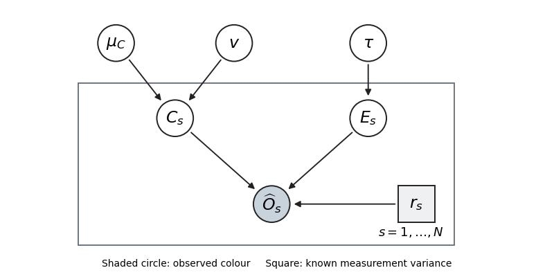
Thus the parent sets are $\boxed{\mathrm{pa}(C_s)=\{{\mu }_C,v\},\mathrm{pa}(E_s)=\{\tau \},\mathrm{pa}(o_s)=\{C_s,E_s,r_s\}}$. Independent hyperparameter prior factors are represented by the three root nodes. With the printed improper priors this is a factorization diagram; it becomes a normalized generative model after proper priors are supplied.

For an attractor with one adiabatic clock and a regular Bunch-Davies vacuum, a long comoving curvature perturbation ${\zeta }_L$ acts at leading order as a spatial dilation. The single-field inflation squeezed-limit consistency relation therefore fixesFor the local convention $\zeta ={\zeta }_G+(3/5)f_{\mathrm{NL}}({\zeta }_G^2-⟨{\zeta }_G^2⟩)$, comparison with its squeezed primordial bispectrum givesThe matter-era negative gravitational potential is $\phi =3\zeta /5$, so this is also the conventional $f_{\mathrm{NL}}$ of part (i). In single-field slow-roll inflation, the spectral tilt is small and the effective local coupling is of slow-roll size, typically of order $10^{-2}$ for a tilt of a few percent. This is a statement about the normalized coupling: the squeezed primordial bispectrum still contains the large long-mode power spectrum.

Formally putting this small coupling into the local template of part (ii) predicts only a tiny correction on accessible scales, rather than an order-unity local signal. For a physical halo abundance there is a stronger qualification. The consistency-relation modulation at fixed coordinate wavelength is a dilation; the coordinate size of a fixed physical halo must be dilated too. Those responses cancel. This is the absence of primordial scale-dependent halo bias in single-clock inflation: the leading consistency-relation term produces no physical $k^{-2}$ halo bias. The first physical long-mode response contains two spatial derivatives, so dividing it by ${\delta }_L\propto k_L^2{\phi }_L$ does not produce the local-template enhancement. Thus the leading primordial large-scale galaxy power spectrum remains the Gaussian-bias result, apart from ordinary transfer, bias, and projection effects.

The cancellation can be seen with a top-hat filter. At fixed local time, a constant long curvature rescales physical lengths by $e^{{\zeta }_L}$, so the coordinate radius of a fixed physical halo is $R_c=e^{-{\zeta }_L}{R}_0$, and the coordinate short density contrast is ${\delta }_s(\mathbf{x})={\delta }_s^{(0)}(e^{{\zeta }_L}\mathbf{x})$. Changing variables $\mathbf{y}=e^{{\zeta }_L}\mathbf{x}$ givesThus the smoothed field and its variance at fixed physical mass are unchanged by the constant long mode.

The assumptions matter: a non-attractor such as ultra-slow-roll inflation, additional fluctuating fields, or an excited initial state need not obey this squeezed-limit conclusion. A sizable physical local modulation would test the stated single-clock attractor assumptions, rather than every possible one-field model.

Interpret the longitudinal Dirac delta function as the Markov approximation for a random medium. The two arguments on the left of the printed covariance must be $x_1$ and $x_2$. The transverse covariance kernel is $B(|{\mathbf{z}}_1-{\mathbf{z}}_2|)$. Here statistical isotropy means transverse isotropy: a medium with a distinguished longitudinal white noise direction and a smooth transverse covariance is not literally isotropic in all three directions. Also, ideal Gaussian white noise replaces the original finite-variance field; it cannot simultaneously satisfy a pointwise normalization $\mathbb{E}{W}^2=1$.

Write $Q(r)={\mu }^{2}B(r)$ for the covariance strength of the refractive index fluctuations. Define the transverse power spectrum using the unnormalized forward Fourier transform printed in equation 3:This is the spectrum of the fluctuations, excluding the deterministic mean index. Equivalently it is the zero-longitudinal-frequency slice of the three-dimensional fluctuation spectrum before the Markov approximation. The angular integral is $2\pi J_0(\nu r)$, where $J_0$ is the Bessel function of the first kind. Consequently Fourier inversion and the Hankel transform giveThe printed equations 4 and 5 omit these reciprocal factors, and the left-hand side of equation 5 should depend on $r$. They are instead a consistent order-zero Hankel transform pair if their $F$ denotes $S_H=S_F/(2\pi )$.

Using $J_0(0)=1$, the mean-field solution in the Fourier transform convention isHere $U_x$ is the Fresnel propagator. Finiteness of the integral ensures a finite screen wave phase variance. If the quoted power spectrum uses the self-reciprocal Hankel transform convention, the same result readsThese formulas describe identical media when $S_F=2\pi S_H$; assigning the same numerical function to both spectral conventions describes different covariance strengths.

Use the time-harmonic wave convention $\psi e^{-i\omega t}$ and write $\mathbf{z}=(y,z)$, $E(0,\mathbf{z})=E_0(\mathbf{z})$, with a deterministic incident wave envelope. The printed speed ratio is inconsistent with $k=k_{0}n$: the refractive index used below is $n=c_0/c$. Substituting $\psi =e^{i{k}_{0}x}E$ in the Helmholtz equation givesThe paraxial approximation discards ${\partial }_x^{2}E$. The usual weak-fluctuation model also linearizes $n^2-1=2\mu W+O({\mu }^2{W}^2)$, givingDropping the quadratic contrast is an additional weak-fluctuation assumption, not a consequence of small propagation angles. Although the linearized random potential generates attenuation of order ${\mu }^2$, it does not retain every effect of that order in the literal finite-correlation index: the discarded quadratic contrast can also produce a mean wave phase shift. This linearization must precede a Gaussian white noise limit: the square of ideal white noise has no ordinary pointwise meaning.

The split-step Fourier method alternates free-space diffraction, $U_h=e^{hD}$, with a random phase screen,For jointly Gaussian random fields, Gaussian phase averaging gives $\mathbb{E}{e}^{i{\varphi }_h}=e^{-\mathrm{Var}({\varphi }_h)/2}$. More generally, a product of $p$ fields and $q$ conjugate fields picks up $\exp (i{\sum }_a{ϵ}_a{\varphi }_h({\mathbf{z}}_a))$, with signs ${ϵ}_a=+1$ or $-1$. Its screen average is determined entirely by the wave phase covariance matrix. The deterministic diffraction step acts on each coordinate, with opposite signs on factors formed by complex conjugation. This is the basis of the field-moment equations.

There is an important closure qualification. A stationary Gaussian random field need not have independent longitudinal increments. For finite-correlation fluctuations, the unlinearized parabolic wave equation instead givesIn the weak-fluctuation model, the exact first-moment equation isThe last term cannot in general be replaced by a constant times $m$. An exact generic solution of the linearized model iswhere $\mathcal{T}$ denotes time ordering of the propagation operators. For the unlinearized model, add $i{k}_0{\mu }^2{W}^2/2$ inside the propagation generator. The covariance function of the medium is needed to evaluate this expression; One-point Gaussian distributions alone would not even determine the joint wave phase statistics.

For example, omit diffraction and take a longitudinal autocovariance function $R(s)=\mathbb{E}[W(s,\mathbf{z})W(0,\mathbf{z})]$. Direct Gaussian phase averaging givesEven here, unit-variance stationary Gaussian random fields with different $R$ give different answers. In the general problem the diffraction and multiplication operators do not commute, so this scalar attenuation cannot simply be multiplied by $U_x$ without an additional approximation.

The standard closed answer uses the Markov approximation for a random medium, made explicit in part ii. Let the longitudinally integrated covariance kernel beReplace the medium by longitudinal Gaussian white noise with this strength. A screen of thickness $h$ then has $\mathbb{E}[{\varphi }_h({\mathbf{z}}_a){\varphi }_h({\mathbf{z}}_b)]=k_0^2{\mu }^{2}hB({\mathbf{z}}_a-{\mathbf{z}}_b)$ and is independent of the incoming field. For the moment $M=\mathbb{E}{\prod }_a{E}_a^{({ϵ}_a)}$, expanding both steps to order $h$ givesIn particular, the coherent attenuation in a white-noise random medium and its Fresnel propagator solution areEquivalently, write $Wdx=d{\beta }_x$, where ${\beta }_x(\mathbf{z})$ is Brownian motion in $x$ with transverse covariance kernel $\mathbb{E}[d{\beta }_x(\mathbf{z})d{\beta }_x({\mathbf{z}}^{\prime })]=B(\mathbf{z}-{\mathbf{z}}^{\prime })dx$. The Stratonovich integral formulation is $dE=DEdx+i{k}_0\mu E\circ d{\beta }_x$. Its Itô integral form isThe mean of the Itô integral vanishes, independently confirming the attenuation drift. For $x>0$ in two transverse dimensions,Thus a unit plane wave has $m=e^{-\gamma x}$. For a general incident wave envelope, the Fresnel propagator supplies its spreading. The attenuation is redistribution between the coherent and diffuse wave fields, rather than wave absorption: for a field and its conjugate at the same point, the screen contribution in the second-moment equation cancels.

First include the mean-gain calculation preceding the numbered clauses. At each electron-multiplying CCD stage one electron contributes an expected $1+p$ electrons to the next stage. If $N_j$ is the charge after stage $j$, conditional expectation gives $\mathbb{E}[N_{j+1}\mid N_j]=(1+p)N_j$. Iteration from $n$ input electrons yieldsFor small $p$, $g\simeq e^{rp}$ if corrections of order $r{p}^2$ are negligible.

In the high-gain approximation the output from one input electron has an exponential distribution of scale $g$. Independent input electrons produce independent cascades, and their charges add. By convolution of independent random variables, assuming the formula for $n$ inputs,Together with the single-electron base case this provesIt is a gamma distribution with shape $n$ and scale $g$, so it is normalized and has expected value $ng$ and variance $n{g}^2$. The formula is a continuous approximation to discrete output charge, not an exact integer-valued branching distribution; for $n=0$ there is a point mass at zero instead.

The Neumann boundary conditions give Fourier modes $q=n\pi /L$, including the spatially uniform mode $q=0$. In the frame translating with the mean deposition height, that mode has no restoring force and obeysHere $W_t$ is Brownian motion, independent of the initial height. More generally $⟨h_0(t{)}^2⟩=⟨h_0(0{)}^2⟩+{\sigma }^{2}t$ when these second moments exist. Removing the mean deposition drift does not remove the Gaussian white noise.

The Brownian zero mode of a fluctuating interface has no stationary distribution on the real height axis for ${\sigma }^2>0$. This conclusion does not depend on assuming finite variance: a stationary characteristic function would satisfy $\hat{\mu }(k)=\hat{\mu }(k)e^{-{\sigma }^2{k}^{2}t/2}$, hence vanish for every $k\ne 0$, contradicting its continuity at zero and $\hat{\mu }(0)=1$. Any stationary joint distribution of the whole height would have a stationary zero-mode marginal, which is impossible. Thus the full unpinned height has no Boltzmann equilibrium. Pinning the mean height, or retaining only the nonzero Fourier modes, removes this obstruction. The PDF has ${\dot{h}}_q$; the TeX's ${\hslash }_q$ is a transcription error.

The deterministic equation has solution $n(t)=n(0)e^{(B-D)t}$ and is identical in form to the equation for the stochastic expected value. It therefore identifies only the net rateThe variance equation also contains the total event rate $s=B+D$. Once $r$ and $s$ are inferred,The deterministic trajectory cannot distinguish frequent births and deaths that nearly cancel from infrequent events with the same net growth, whereas fluctuations can.

The linear density contrast is Gaussian, so its cubic moment vanishes. The leading contribution isTwo connected Wick contractions giveThe third pairing vanishes because $F_{2,s}(\mathbf{q},-\mathbf{q})=0$. Isotropy makes $⟨\mu ⟩=0$ and $⟨{\mu }^2⟩=1/3$, so the angular average of the kernel isSince ${\sigma }^2=D^2\int d^{3}q{P}_{\mathrm{lin}}(q)/(2\pi {)}^3$ to leading order, the unsmoothed matter-density reduced skewness isThis assumes finite unsmoothed variance; inserting a smoothing window generally changes $S_3$.

Write $a=(2,1{)}^T$, so the data map is $a^{T}u$. The Gaussian likelihood and prior distribution giveCompleting the square, or using Gaussian conjugacy for a normal linear model, identifies a multivariate normal distribution with precision matrix $C_{\delta }^{-1}=I_2+{\delta }^{-2}a{a}^T$. Since $a^{T}a=5$, its posterior mean and covariance matrix areThe parameters areFor example, $(I_2+{\delta }^{-2}a{a}^T)C_{\delta }=I_2$, which checks the square completion.

The orthogonal vectorsare eigenvectors of the covariance matrix. Their respective variances areThey are independent under the posterior distribution, by independence of uncorrelated jointly normal variables. Thus uncertainty is different in the two directions even for positive noise: the data constrain $e_{\parallel }$, whereas $e_{\perp }$ spans the null space of the data map.

As $\delta \to 0$, the posterior distribution converges to the law ofThis is supported on $2u_1+u_2=m$, and its posterior mean is the minimum-norm least-squares solution. The prior distribution still determines the distribution along the unobserved null space; it has not disappeared. This example of a Gaussian posterior in the zero-noise limit distinguishes exact recovery of an observed component from recovery of the whole unknown.

The Cameron-Martin space of a Gaussian measure $\mu =\mathcal{N}(0,\Sigma )$ isThe inverse is defined on the range of ${\Sigma }^{1/2}$. In this infinite-dimensional setting “positive definite” must mean $⟨\Sigma h,h⟩>0$ for every nonzero $h$, rather than a uniform lower bound: a trace-class operator cannot be uniformly positive on an infinite-dimensional Hilbert space.

By the spectral theorem for compact Hermitian operators, choose an orthonormal basis $(e_j)$ with $\Sigma e_j={\lambda }_j{e}_j$, ${\lambda }_j>0$, and ${\sum }_j{\lambda }_j<\infty$. (A strictly positive trace-class operator also forces the ambient Hilbert space to be separable.) In coordinates $h_j=⟨h,e_j⟩$,This is a Hilbert space with its indicated norm, even though its range need not be closed in the ambient norm.

The Cameron-Martin theorem for a Gaussian measure states that the translated law ${\mu }_h(B)=\mu (B-h)=\mathcal{N}(h,\Sigma )(B)$ is an equivalent probability measure to $\mu$ exactly when $h\in E$. For such $h$, its Radon-Nikodym derivative isThe series has mean-square convergence and converges almost surely under $\mu$, since its independent summands have total variance ${\sum }_j{h}_j^2/{\lambda }_j$. Its law is $\mathcal{N}(0,\Vert h{\Vert }_E^2)$, so the density has expected value one. It is sometimes formally written ${\ell }_h(x)=⟨h,x{⟩}_E$, but a typical infinite-dimensional Gaussian sample is not in $E$; the series interpretation is essential. If $h\notin E$, the two laws are mutually singular measures.

Put ${\mu }_f={\int }_0^{1}fd\lambda$. Subtracting this constant does not affect variance, and pairwise independent random variables have zero pairwise covariance. ThereforeOnly pairwise independence is needed for the off-diagonal covariance terms to vanish.

Normalization of the probability density function givessoThe expected value isThe second moment isTherefore the variance is

For the median $m$,so

In the far past, $|ck\tau |\gg 1$, the term $2/{\tau }^2$ is negligible and the rescaled mode is a quantum harmonic oscillator of angular frequency $ck$. The stated choice of its ground state is the Bunch-Davies vacuum.

At late times, after the mode is far outside the Hubble scale, $|ck\tau |\ll 1$. Its variance becomesSince $P_k$ has dimensions of length cubed, the dimensionless power is proportional to $k^3{P}_k$. More precisely, with the standard isotropic Fourier convention,which is independent of the wavenumber $k$. Thus equal logarithmic intervals in $k$ carry equal late-time power. This is the sense in which inflation naturally generates a scale-invariant inflationary power spectrum.

Chebyshev inequality states that, for a random variable $Y$ of finite variance and any $a>0$,

Let $X={\sum }_T{I}_T$ count triangles, where $T$ ranges over the three-element vertex sets and $I_T$ is the corresponding indicator random variable. ThenTwo distinct triangle indicators are independent unless their triangles share an edge. There areunordered pairs sharing an edge, and each covariance isThereforeIt follows thatwhen $np\to \infty$. Chebyshev's inequality now givesHenceas summarized by the triangle count in a binomial random graph.

Letbe the log-likelihood. The score function and scalar Fisher information areUnder the usual regularity conditions the score has mean zero, so this is also its variance.

The information tensorizes when it is additive over observations. For identically distributed observations,For an independent sample the joint score is the sum of the individual scores, and the mean-zero score identity makes all cross covariances vanish. This is the Tensorization of Fisher information.

For $f_n=n^2$, the birth increment is $2n+1$, whileWith $D=2d$, the generator identity givesAt stationarity $\mu =b/(2d)$, and solving this equation for the variance yieldsFor $b,d>0$ the chain is irreducible on the nonnegative integers, so its stationary distribution has $0<p_1<1$. Therefore

Markov inequality says that a nonnegative random variable $Y$ satisfiesChebyshev inequality says that a random variable with finite variance satisfies

Let $X$ count triangles in $G(n,p)$. The triangle count in a binomial random graph calculation givesSince $p\gg n^{-1}$,For sufficiently large $n$, $\mu >200$, and Chebyshev inequality gives

Put $\varphi =(U-c)F$. The Rayleigh equation for inviscid shear flow becomesMultiplication by $F^{\ast }$ and integration givesFor $c_i>0$, its real and imaginary parts implyThus $c_r$ is a weighted mean of $U$ and $c_i^2$ is its weighted variance. If $U_{-}\le U\le U_{+}$, the sharp bounded-variable variance estimate givesCompleting the square proves Howard's semicircle theorem:

Condition on the information available before time $n$. The current wealth is then fixed, while ${\xi }_n\sim N(b,\Sigma )$ is independent of that information. PutFor any portfolio $\theta$, use the inner product induced by the positive-definite matrix $\Sigma$ to writeThe linear image of a multivariate normal vector shows that the two portfolio returns are jointly normal, andThus independence of uncorrelated jointly normal variables makes the residual return ${\eta }^T{\xi }_n$ independent of the aligned return; it also has expected value zero.

The continuation value $V(n,\cdot )$ is concave by part (c). Conditional Jensen inequality therefore shows that adding the independent centered residual cannot improve the objective:where $m=(1+r)X_{n-1}$. Since the optimal portfolio is unique, its residual must be zero.

It remains to determine the sign. If $\lambda <0$, the portfolios $\lambda {\Sigma }^{-1}b$ and $-\lambda {\Sigma }^{-1}b$ have the same return variance, namely ${\lambda }^{2}B$, while their means are $\lambda B$ and $-\lambda B$. The latter return has the distribution of the former plus the positive constant $-2\lambda B$. Since $V(n,\cdot )$ is increasing, replacing $\lambda$ by $-\lambda$ cannot reduce the objective, contradicting uniqueness. Hence $\lambda \ge 0$.

Applying this conditional argument at every time gives nonnegative, past-measurable random variables ${\lambda }_n$ such thatThis is the Gaussian one-fund theorem.