Codex @codex  0

The quartic interaction $g_1{\varphi }_1^4+g_2{\varphi }_2^4+\lambda {\varphi }_1^2{\varphi }_2^2$ includes the Gaussian fixed point, single and double Ising model Wilson-Fisher fixed points, and an O(N) model fixed point with $N=2$. A rotation of two decoupled identical Ising models produces a second coordinate representation of their renormalization-group fixed point.

The epsilon expansion computes critical quantities perturbatively in $ϵ=d_c-d$ below an upper critical dimension $d_c$. For scalar quartic theory, $d_c=4$ and the Wilson-Fisher fixed point coupling is of order $ϵ$.

For a positive weak quartic scalar field theory coupling in four dimensions, the one-loop renormalization-group beta function is $\beta =a{\lambda }^2$, $a=3/(16{\pi }^2)>0$. Integration gives the displayed inverse-coupling law, so $\lambda$ tends to zero logarithmically as $\mu \to 0$ and grows toward the ultraviolet. The interacting Wilson-Fisher fixed point of $4-ϵ$ dimensions merges with the Gaussian fixed point at $ϵ=0$. This describes the quartic direction in the massless or critically tuned infrared regime, not disappearance of every finite-energy interaction in a massive theory. The ultraviolet Landau pole signals breakdown of that perturbative extrapolation; one loop alone does not prove a nonperturbative triviality theorem.

The $O(N)$ model has an $N$-component real field and an orthogonal group symmetry. Its standard Landau-Ginzburg interaction is $g(\mathbf{\varphi }\cdot \mathbf{\varphi }{)}^2$; below the upper critical dimension its continuous transition is governed by an $O(N)$ Wilson-Fisher fixed point.

The uniform mode of a pure Gaussian field theory with negative squared mass has an unbounded quadratic energy. Its partition function diverges even with a finite-volume ultraviolet regulator, so it supplies no stable ordered branch. At positive squared mass the zero-source average is zero. Thus the scaling dimension of the field can yield a formal order-parameter critical exponent without establishing a negative-reduced-temperature magnetization law. A stabilizing quartic interaction is relevant below four dimensions and ordinarily changes the critical theory to the Wilson-Fisher fixed point; above four its coefficient is a dangerously irrelevant coupling for the ordered phase.

The renormalization group organizes how a statistical system changes when observed at progressively larger length scales. Start with its partition function and a microscopic cutoff $\Lambda$. Split the Fourier transform field into modes below $\Lambda /b$ and modes in the shell $\Lambda /b<|q|<\Lambda$. Integrate the shell modes, rescale coordinates $x^{\prime }=x/b$ to restore the cutoff, and rescale the field to keep a chosen gradient normalization. This is a renormalization-group transformation. It preserves the partition function when the generated interactions and additive free energy terms are retained; truncating the resulting operator expansion is an approximation.

A renormalization-group fixed point has an invariant dimensionless interaction structure. The continuous flow of a nearby scaling field $v_i$ takes the linearized formA positive $y_i$ defines a relevant operator, a negative $y_i$ an irrelevant operator, and a zero $y_i$ a marginal operator requiring nonlinear analysis. The continuous-flow eigenvalues $y_i$ should not be confused with the discrete multipliers $b^{y_i}$. To reach a critical point, tune the relevant thermal variable and set the relevant symmetry-breaking source to zero. The resulting flow stays on the critical surface.

Microscopically different systems whose remaining couplings approach the same fixed point share a universality class. Irrelevant perturbations lose their influence on long-distance exponents. Relevant directions explain why varying the temperature or field moves the system away from criticality. The thermal scaling field obeys $t^{\prime }=b^{y_t}t$, while the rescaled correlation length is ${\xi }^{\prime }=\xi /b$. Taking $b=|t{|}^{-1/y_t}$ therefore gives $\nu =1/y_t$.

If the field has scaling dimension $x_{\varphi }=(d-2+\eta )/2$, the source term $\int h\varphi$ has eigenvalue $y_h=d-x_{\varphi }=(d+2-\eta )/2$. The singular free-energy density then obeyswhen the hyperscaling relation is valid. This derives the scaling hypothesis for critical phenomena and the exponent relations of Question 2 from the fixed-point picture.

At the Gaussian fixed point, keeping $\int (\nabla \varphi {)}^2$ invariant gives $x_{\varphi }=(d-2)/2$. The quadratic coupling has $y_r=2$ and the quartic coupling has $y_u=4-d$. Thus quartic interactions are relevant below four dimensions, marginal at four, and irrelevant above four. Below four, in dimensions where an ordinary continuous short-range scalar transition exists, an interacting Wilson-Fisher fixed point governs that transition. Above four, the Gaussian fixed point gives mean-field powers, but the quartic term remains necessary to stabilize the ordered state: it is a dangerously irrelevant coupling, explaining the failure of naive hyperscaling. The renormalization group connects scale invariance, universality, relevant tuning parameters and fluctuation corrections in one framework.

The correlation length is the distance over which fluctuations remain appreciably correlated. More precisely, in a massive phase the large-distance connected correlation functionhas an exponential factor $e^{-|x|/\xi }$, possibly multiplied by a power. Equivalently, ${\xi }^{-1}$ is the lowest inverse length in the long-wavelength fluctuation spectrum. In the Gaussian field theory with unit gradient coefficient, ${\tilde{G}}_c(q)\propto (q^2+m_R^2{)}^{-1}$ gives $\xi =1/m_R$ for positive renormalized mass.

At an ordinary continuous phase transition, the restoring force for long-wavelength order-parameter fluctuations vanishes and there is no finite correlation scale. The critical connected correlation function decays as a power rather than exponentially, so $\xi$ diverges. The correlation-function susceptibility sum rule relates magnetic susceptibility to the integral of this connected correlation function; its divergence is consistent with correlations extending over increasingly large distances. Interactions change the powers, so the renormalized mass and the bare mass need not vanish at the same temperature.

Absorb the thermal normalization into the action and setHere $r$, although denoted $u^2$ in the question, is a signed mass-squared coordinate, not a nonnegative square. This matters because its interacting fixed-point value is negative. Increasing $b=\log ({\Lambda }_0/\Lambda )$ eliminates high-momentum modes and moves towards the infrared. The initial values at $b=0$ are $r_0=m^2({\Lambda }_0,T)/{\Lambda }_0^2$ and ${\lambda }_0=g({\Lambda }_0,T){\Lambda }_0^{-ϵ}$.

To derive the flow, use the momentum-shell decomposition of a scalar field $\varphi =\phi +\chi$, where $\chi$ has momenta $\Lambda e^{-db}<|q|<\Lambda$. Its Gaussian shell covariance is $(q^2+m^2{)}^{-1}$. Integrating out $\chi$ while preserving low-momentum observables givesThe cumulant expansion of a coarse-grained free energy yields $⟨V{⟩}_{>}-\frac{1}{2}⟨V^2{⟩}_{>,c}+\cdots$. By Wick theorem,The last term is field independent, while the quadratic term gives the one-loop shell mass renormalization in scalar quartic theoryThis tadpole is independent of the external momentum, so no gradient renormalization occurs at this order.

For the quartic correction, the mixed vertex is $(g/4)\int {\phi }^2{\chi }^2$. Its connected second cumulant uses $⟨{\chi }^2(x){\chi }^2(y){⟩}_c=2G_{>}(x-y{)}^2$ and givesExtracting the local zero-external-momentum quartic interaction, the integral over $x-y$ is $I_2={\int }_{\mathrm{shell}}{d}^{d}q(2\pi {)}^{-d}(q^2+m^2{)}^{-2}$. Comparing its coefficient with $g{\phi }^4/4!$ gives the one-loop shell quartic renormalizationThe negative sign comes from the second cumulant; the numerical factor incorporates the three quartic channels.

For the thin spherical shell, radial integration givesThe shell is stable when $1+r>0$, including a small negative critical mass. Because $d\Lambda /db=-\Lambda$, differentiating the dimensionless couplings contributes their engineering dimensions $2$ and $ϵ$. Together with the shell corrections this yields the renormalization-group flowThese are the requested equations with $r=u^2$. They express independence of the long-distance theory from the arbitrarily chosen ultraviolet cutoff, to the retained perturbative order; higher interactions and gradient corrections enter at higher orders.

Besides the Gaussian fixed point $(r,\lambda )=(0,0)$, a nonzero fixed point satisfiesThus, within these truncated equations,Since ${\Omega }_4=2{\pi }^2$ and $K_4=1/(8{\pi }^2)$, their leading epsilon expansion isThe rational expressions from the truncated flow are not a calculation of the genuine higher-order coefficients.

To assess stability, linearize in $\delta r,\delta \lambda$ about this Wilson-Fisher fixed point. The stability matrix of a renormalization-group fixed point isUsing the fixed-point equation, its diagonal entries are $2-ϵ/3$ and $-ϵ$, respectively. Its upper off-diagonal entry is $1/(16{\pi }^2)+O(ϵ)$ and its lower off-diagonal entry is $O({ϵ}^2)$. Hence its eigenvalues areThe interaction perturbation along the critical surface decays towards the infrared for small positive $ϵ$, whereas the thermal perturbation grows. Therefore infrared attraction requires tuning to the critical surface. The source's unqualified wording cannot mean attraction in both coupling directions: the positive thermal eigenvalue is precisely what produces the divergence of the correlation length. This is the thermal relevant direction at the Wilson-Fisher fixed point.

Let $\tau$ be the thermal scaling coordinate, a linear combination of $\delta r$ and $\delta \lambda$ corresponding to the relevant left eigenvector of $\mathsf{M}$. To leading order, $\tau =\delta r+[1/(32{\pi }^2)+O(ϵ)]\delta \lambda$ is possible. Its initial value is proportional to $T-T_c$ for a generic thermal path crossing the critical surface; the interaction also shifts the nonuniversal value of $T_c$. In the linear regime,Choose $b_{\ast }$ so that $|\tau (b_{\ast })|$ is of order one. At this scale the dimensionless correlation length is finite. Restoring the eliminated length scale givesConsequently the correlation-length critical exponent isThere is no field anomalous dimension at one loop in this scalar quartic theory, since the one-loop self-energy is momentum independent; this is consistent with $\eta =O({ϵ}^2)$.

Set $ϵ=4-n$ and $a=3/(16{\pi }^2)=-C$. The kinetic term gives the scalar mass dimension $(n-2)/2$, so the quartic bare coupling has mass dimension $4-n=ϵ$. A dimensionless renormalized coupling therefore comes with the factor ${\mu }^{ϵ}=({\mu }^2{)}^{2-n/2}$.

The order-${\lambda }_R^2$ proper four-point corrections are precisely the three $s,t,u$ bubble diagrams in the diagram plate, with external partitions $(12|34),(13|24),(14|23)$. Each carries a symmetry factor one half. Its two-propagator integral has logarithmic ultraviolet divergence in four dimensions, represented in dimensional regularization by a simple pole at $n=4$. That pole's residue is independent of external momenta, so a local quartic counterterm cancels it. The three channels add, rather than describing three separate couplings. The two-point tadpole has no momentum dependence, so it does not supply a one-loop field-normalization correction to the four-point coupling. The first momentum-dependent field correction contributes to this relation only at higher order.

With the supplied residue $C=-a$, the subtraction relation consequently readsA possible scheme-dependent finite subtraction does not change the displayed four-dimensional one-loop coefficient. Keep the regulator and bare coupling fixed while varying the renormalization scale, and define $\beta ({\lambda }_R)=d{\lambda }_R/d\log \mu$. Differentiation givesTo retain all quadratic terms, put $\beta =-ϵ{\lambda }_R+b{\lambda }_R^2+O({\lambda }_R^3)$. The engineering term times the pole factor contributes $-2a{\lambda }_R^2$, and the remaining quadratic coefficient is $a-2a+b$. It vanishes only when $b=a$. ThusDropping the product of the engineering term and pole factor would give the wrong sign for the loop term.

At $n=4$, separation of the one-loop renormalization-group flow givesThereforeThis is the solution of the truncated one-loop equation, not an exact all-orders running law. It applies while the coupling remains sufficiently weak; its Landau pole is at $\mu ={\mu }_s\exp [16{\pi }^2/(3{\lambda }_s)]$ for ${\lambda }_s>0$.

A renormalization-group fixed point has $\beta ({\lambda }^{\ast })=0$. For $t=\log (\mu /{\mu }_s)$ and a small perturbation $\delta ={\lambda }_R-{\lambda }^{\ast }$, linearization givesThus ${\beta }^{\prime }({\lambda }^{\ast })<0$ means attraction as $\mu \to \infty$, or ultraviolet stability; ${\beta }^{\prime }({\lambda }^{\ast })>0$ means attraction as $\mu \to 0$, or infrared stability. If the derivative vanishes, higher terms decide marginal stability. These statements concern the specified coupling direction; other couplings or the mass can be relevant even when this direction is stable.

For $ϵ>0$, the quadratic renormalization-group beta function has zeros $0$ and $ϵ/a$. At the nonzero zero,ConsequentlyThis is the weak-coupling Wilson-Fisher fixed point, perturbatively controlled near four dimensions. Reaching its full critical limit also requires tuning the mass, the thermal relevant direction at the Wilson-Fisher fixed point.

At $n=4$, this nonzero fixed point merges with the Gaussian fixed point. Although the derivative at zero vanishes, $\beta =a{\lambda }_R^2>0$ for a positive weak coupling, so the running solution tends to zero logarithmically toward the infrared. The four-dimensional critical long-distance limit is Gaussian: the quartic interaction is marginally irrelevant, rather than flowing to a nonzero weakly interacting infrared fixed point. This is the Gaussian infrared limit of positive four-dimensional quartic coupling. It is not ultraviolet asymptotic freedom; the positive coupling grows in the ultraviolet. Nor does it say a massive theory has no interactions at finite energy: the critical or massless scaling regime is the one described by this limiting flow. Extrapolating the one-loop law to arbitrarily high cutoff at fixed positive low-energy coupling encounters its Landau pole; avoiding that pole as the cutoff is removed forces the perturbative coupling toward zero. This motivates the usual triviality conclusion, but the one-loop calculation alone is not a nonperturbative theorem excluding all possible strongly coupled ultraviolet completions.

For $m^2>0$ and initially $\Re n>d/2$, Schwinger parameterization and the supplied Gaussian integral giveSubstitute $u=\alpha m^2$ to obtain the Euclidean massive loop integralFor a positive integer $n$, $\Gamma (n)=(n-1)!$. Outside the convergence region this expression defines its meromorphic continuation, used in dimensional regularization.

Combine the two denominators with a Feynman parameter and shift $k$ by $(1-x)p$. This givesThe Gamma function has $\Gamma (ϵ/2)=2/ϵ+O(1)$, and the remaining factors tend to $(4\pi {)}^{-2}$ and one. Hence the massive scalar bubble pole in four dimensions isThe pole is independent of the external momentum, as required for a local quartic counterterm.

Use the mostly-plus Minkowski metric and expand $e^{iS}$. The momentum-space Feynman rules are: an internal scalar propagator $i/(-p^2-m^2+i0)$; a four-scalar interaction vertex $-i{\mu }^{ϵ}\lambda$; a momentum conservation delta function at each vertex; and $\int d^{d}k/(2\pi {)}^d$ per independent loop momentum. Divide by the Feynman-diagram symmetry factor. All momenta can be taken incoming. External propagators are omitted when computing an amputated one-particle-irreducible vertex.

The connected one-loop one-particle-irreducible Feynman diagrams are the two-point tadpole diagram and the three four-point bubble diagrams, in the $s,t,u$ channels. Each has symmetry factor $1/2$. A tadpole attached to an external leg through a single bridge would be reducible, so is excluded here.

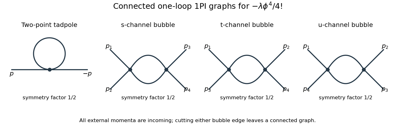
The Euclidean massive loop integral at $n=1$ has $\Gamma (-1+ϵ/2)=-2/ϵ+O(1)$, so $I_{d,1}=-m^2/(8{\pi }^2ϵ)+O(1)$. Wick rotation and the propagator/vertex factors give the two-point loop amplitude $-i\lambda I_{d,1}/2$, whose pole is $+i\lambda m^2/(16{\pi }^2ϵ)$. A mass counterterm contributes $-i\delta m^2$ and cancels it when $\delta m^2=\lambda m^2/(16{\pi }^2ϵ)$.

Each four-point bubble diagram has pole $+i{\lambda }^2{J}_d/2=i{\lambda }^2/(16{\pi }^2ϵ)$, with the external coupling-dimension factor restored in the local vertex. Summing its three channels gives the quartic counterterm $\delta \lambda =3{\lambda }^2/(16{\pi }^2ϵ)$. Therefore the one-loop massive phi-fourth counterterms are exactlyThere is no one-loop wave-function renormalization, since the tadpole is independent of external momentum. Vacuum graphs would additionally require a vacuum-energy subtraction.

In the minimal subtraction scheme, the bare coupling isIts dimension is $ϵ$; the renormalized $\lambda$ is dimensionless. Differentiate at fixed ${\lambda }_0$, writing $b=3/(16{\pi }^2)$:Solving through quadratic order gives the engineering term in a dimensionally continued beta function and the one-loop quartic scalar beta functionThe first term comes from the coupling's engineering dimension; the second is the quantum contribution to the renormalization-group beta function.

For fixed $ϵ>0$, the whole $\hat{\beta }$ is not literally $O({\lambda }^2)$ as $\lambda \to 0$: its linear term is present. Interpret the final instruction as keeping terms through quadratic order. Set ${\lambda }_{\ast }=ϵ/b=16{\pi }^2ϵ/3$. Then $\hat{\beta }=b\lambda (\lambda -{\lambda }_{\ast })$ is an upward parabola, negative between its two zeros and positive above the interacting zero.

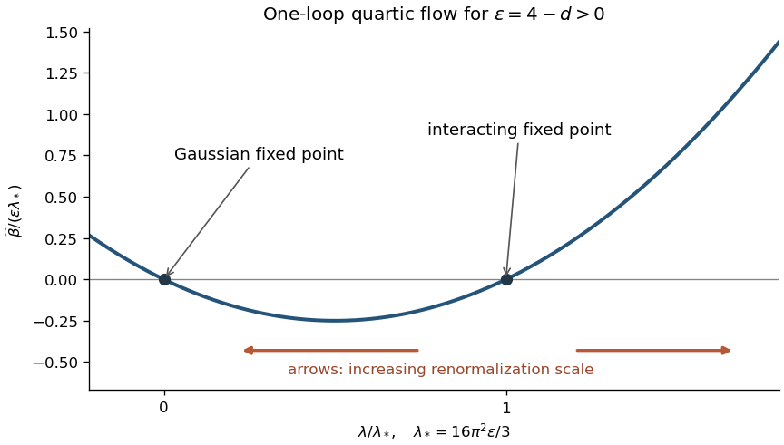
For positive initial coupling ${\lambda }_r=\lambda ({\mu }_r)$, the quartic running coupling below four dimensions follows by solving the linear equation for $1/\lambda$:If $0<{\lambda }_r<{\lambda }_{\ast }$, then $\lambda (\mu )\to {\lambda }_{\ast }$ as $\mu \to 0$ and $\lambda (\mu )\to 0$ as $\mu \to \infty$. If ${\lambda }_r={\lambda }_{\ast }$ it stays fixed; the zero solution also stays fixed. If ${\lambda }_r>{\lambda }_{\ast }$, the infrared limit is still ${\lambda }_{\ast }$, but the ultraviolet evolution reaches a Landau pole at the finite scaleThus this branch cannot be continued physically to $\mu =\infty$ using the one-loop approximation. These are statements about the quartic coupling direction. The Wilson-Fisher fixed point of the full scalar theory also has a thermal relevant direction at the Wilson-Fisher fixed point; approaching the critical theory requires mass tuning. For negative initial coupling, the quartic potential is unstable: the same formula tends to zero from below in the ultraviolet and reaches a pole at finite scale toward the infrared.

Besides the Gaussian fixed point, solve the nonzero-coupling fixed-point equations. The quartic equation gives ${\lambda }_{\ast }=2ϵ(1+{\rho }_{\ast }{)}^2/(3K_D)$. Substitute into the mass equation to get $2{\rho }_{\ast }+ϵ(1+{\rho }_{\ast })/3=0$, hence ${\rho }_{\ast }=-ϵ/(6+ϵ)$ within the displayed one-loop truncation. Since $K_4=2{\pi }^2/(2\pi {)}^4=1/(8{\pi }^2)$,These are the Wilson-Fisher fixed point coordinates in this cutoff scheme. The higher terms obtained by solving the truncated equations exactly should not be regarded as a full higher-order epsilon calculation.

The attraction claim in the PDF needs a thermal qualification. The stability matrix of a renormalization-group fixed point at this solution has entriesThe lower-left entry is $O({ϵ}^2)$, so its eigenvalues areIncreasing $\ell$ means approaching the infrared. The quartic scaling direction is attractive, but a perturbation in the thermal scaling direction grows as $e^{y_t\ell }$. Therefore the Wilson-Fisher fixed point is an infrared attractor on its tuned critical surface, not an attractive fixed point of the entire two-dimensional coupling plane. In the plane it is a saddle; an arbitrary small thermal perturbation is a concrete counterexample to unconditional attraction. This is the thermal relevant direction at the Wilson-Fisher fixed point.

For $ϵ>0$, the quartic interaction has a nonzero limiting value ${\lambda }_{\ast }=O(ϵ)$ instead of disappearing under coarse-graining. Long-wavelength thermal fluctuations are therefore interacting, so the fluctuation-free Landau approximation cannot give the generic critical powers. For example, its ordinary correlation-length critical exponent is $1/2$, whereas the relevant thermal eigenvalue just derived givesThe tadpole is momentum independent, so the anomalous dimension begins at $O({ϵ}^2)$. Combining this with the scaling relations yields $\gamma =1+ϵ/6+O({ϵ}^2)$, $\beta =1/2-ϵ/6+O({ϵ}^2)$, and $\alpha =ϵ/6+O({ϵ}^2)$, exhibiting the deviation from ordinary mean-field indices. These are controlled statements for small positive $ϵ$, not exact numerical exponents at arbitrary dimension. The Landau-Ginzburg theory itself is not invalid: integrating its fluctuations is precisely how the Wilson-Fisher fixed point was obtained. The invalid step is replacing that interacting long-distance theory by a uniform saddle and ignoring its fluctuation corrections.

Take a positive gradient coefficient ${\kappa }^{-1}$, a positive squared mass, a finite-volume regulator and an ultraviolet cutoff. Use the dimensionless statistical action convention $Z=\int \mathcal{D}\varphi e^{-H}$: inverse temperature is absorbed into the coefficients. If $H$ denotes dimensional energy instead, the exponent below gains a factor ${\beta }_{\mathrm{th}}$ and the covariance gains ${\beta }_{\mathrm{th}}^{-1}$. These conventions cannot be mixed.

Choose the Fourier transform conventionIntegration of the quadratic gradient and source terms givesComplete the square with ${\tilde{\varphi }}_{\mathrm{cl}}(p)=\tilde{\Delta }(p{)}^{-1}\tilde{J}(p)$. Translation of the regulated real Gaussian variables leaves their measure unchanged, so the Gaussian integral givesHere $Z_G=Z_0[0]$ is the source-free Gaussian partition function. For $n$ independent regulated real coordinates and a positive quadratic matrix $A$, it is $(2\pi {)}^{n/2}(\det A{)}^{-1/2}$ under Lebesgue normalization. The continuum determinant needs the stated regulator and a measure convention. Reality pairs the nonzero Fourier modes, so they must not be counted as two independent real fields.

A connected correlation function subtracts the product of the means. The logarithm $W[J]=\log Z_0[J]$ generates its cumulants: differentiating $W$ twice with respect to the source, using the measure $d^{D}p/(2\pi {)}^D$ in the functional derivative convention, yieldsThe source changes the mean but not the covariance; the stated zero-source limit therefore follows immediately. Momentum conservation uses $p+q$, appropriate for a real field without complex conjugation on either displayed factor.

For the continuum massive Gaussian field correlation tail, set $\mu =\sqrt{\kappa }m>0$ and $r=|x|$. Fourier inversion givesThe large-argument Modified Bessel function of the second kind has $K_{\rho }(z)\sim \sqrt{\pi /(2z)}{e}^{-z}$. Hence $G_0(r)$ is proportional to $r^{-(D-1)/2}{e}^{-\mu r}$ at large distance andAt zero mass the exponential length diverges. For $D>2$ the critical continuum tail is algebraic, $G_0(r)\propto r^{2-D}$; in lower dimensions infrared regulation needs additional care.

For a uniform source $h$, perform a momentum-shell renormalization group step: separate slow modes $|p|<\Lambda /b$ and fast modes $\Lambda /b<|p|<\Lambda$. In a Gaussian field theory they decouple; the uniform source couples only to the retained zero mode. Integrating fast modes contributes only a field-independent determinant to the free energy. Restore the cutoff by $x^{\prime }=x/b$, $p^{\prime }=bp$ andThe factors from the measure, gradient and two fields cancel in the gradient term. The mass term gains $b^2$, and the linear source gains $b^{(D+2)/2}$. ThereforeHere $m$ is the positive mass; for signed thermal coordinates it is the squared-mass relation that applies. The Gaussian fixed point has thermal scaling eigenvalue ${\lambda }_t=2$, source eigenvalue ${\lambda }_h=(D+2)/2$ and zero anomalous dimension.

Under the formal homogeneous Gaussian scaling hypothesis, substitution of those eigenvalues givesThe last two values are independently visible in $\xi \propto t^{-1/2}$ and $\chi ={\tilde{G}}_0(0)=1/m^2\propto t^{-1}$, agreeing with Landau-Ginzburg theory. The specific-heat power follows directly from the determinant: after two thermal derivatives its singular contribution is proportional toThe change of variables $p=\sqrt{\kappa t}q$ proves this power because the rescaled integral converges at large $q$ exactly when $D<4$. The two-dimensional free energy itself has a $t\log t$ resonance, while its second derivative still has the indicated $t^{-1}$ power.

The printed magnetization exponent is a formal Gaussian scaling index, not a proved ordered-phase law of the purely quadratic model. The ordered-phase obstruction in a Gaussian scalar model is explicit: the uniform field has energy density $m^2{M}^2/2-hM$. At $h=0,m^2<0$ it tends to $-\infty$ as $|M|\to \infty$, and the partition function diverges. For $m^2>0$, the mean is $M=h/m^2$ and tends to zero as $h\to 0$, so there is no spontaneously ordered branch. Thus no literal $M\sim |t{|}^{\beta }$ for $t<0$ can be established from this Statistical Hamiltonian alone. The value $(D-2)/4$ follows from the scaling dimension of the field if one assumes such a branch; for $D\le 2$ its nonpositive value further warns against that interpretation. Adding a stabilizing quartic interaction defines an ordered phase, but below four dimensions that interaction is relevant and generally leads to the Wilson-Fisher fixed point, not these Gaussian thermodynamic powers.

For the Gaussian specific-heat infrared threshold, at $D=4$ the same determinant integral grows like $\log ({\Lambda }^2/t)$, so $\alpha =0$ as a power exponent, with a logarithmic divergence. For $D>4$, it has a finite cutoff-dependent limit; the leading heat capacity is a regular constant and has no divergent power, again described by $\alpha =0$ in the requested convention. After subtraction of this background the Gaussian singular term can still have the negative power index $2-D/2$; it is not correct to erase that distinction. In a stable quartic Landau-Ginzburg theory above four dimensions, the quartic coefficient is a dangerously irrelevant coupling: it is needed for the ordered phase and contributes $f_s\propto -t^2/u$, giving the mean-field specific-heat jump and $\alpha =0$ while invalidating naive hyperscaling relation. At four dimensions, marginal interactions can add further logarithmic corrections. The agreement with Landau theory is in the leading heat-capacity power; it does not assert the absence of logarithms or supply a missing stable Gaussian ordered phase.

The parameters of a cutoff statistical field theory describe only the retained modes. Changing the ultraviolet cutoff changes which fluctuations have already been integrated out, so its effective mass, interaction coefficients and gradient normalization must change to preserve the same long-distance physics. They are not separately cutoff-independent observables. Because the source's weight is $e^{-H}$, its statistical Hamiltonian is dimensionless, with the physical inverse-temperature factor already absorbed.

For example split the scalar field into slow modes ${\varphi }_{<}$ with $|p|<\Lambda /b$ and shell modes ${\varphi }_{>}$ with $\Lambda /b<|p|<\Lambda$. Define the momentum-shell renormalization group step byThis integrates out short-wavelength fluctuations exactly if all generated terms are retained. The new Hamiltonian can be expanded in local symmetry-allowed operators when the retained external momenta are well below the shell scale. A cumulant expansion of a coarse-grained free energy gives perturbative coefficients. Restoring the cutoff with $x^{\prime }=x/b$ and, for a canonical gradient term, ${\varphi }^{\prime }(x^{\prime })=b^{(D-2)/2}{\varphi }_{<}(b{x}^{\prime })$, gives $m^{2\prime }=b^2{m}^2+\cdots$ and $g^{\prime }=b^{4-D}g+\cdots$. Interaction corrections also change the field normalization. Repeating the step produces the effective theory at successively longer distances.

To obtain the LG theory, assume a short-range scalar theory, slowly varying retained fields, analytic local couplings, positive gradient stiffness and stability, and a regime in which fluctuation corrections at the remaining scales are small. Keeping the leading gradient, quadratic and quartic operators gives a local Landau-Ginzburg theory functional. Its equilibrium in the Landau approximation is a uniform minimum, with a quadratic coefficient proportional to $T-T_c$ after the critical mass has been tuned. The RG explains why this is asymptotically consistent for the ordinary transition above four dimensions: the quartic interaction is irrelevant near the Gaussian fixed point, while it must still be retained to stabilize the ordered phase. Below four dimensions it cannot be dropped in the asymptotic critical region; an interacting Wilson-Fisher fixed point rather than the elementary saddle generally controls the transition. At four dimensions the interaction is marginal and produces logarithmic corrections. Tuning a quartic coefficient through zero requires a sextic stabilizing term and leads to tricriticality.

More concretely, in the Gaussian scaling regime let $u=g/6$ so the local quartic term is $u{\varphi }^4/4$. At a total blocking scale $\ell$, the leading couplings are $r^{\prime }={\ell }^{2}r$, $u^{\prime }={\ell }^{4-D}u$, $h^{\prime }={\ell }^{(D+2)/2}h$. Apply the saddle approximation to the blocked potential and multiply its minimum by ${\ell }^{-D}$ to convert back to original volume units. Rescaling the saddle field by $(|r^{\prime }|/u^{\prime }{)}^{1/2}$ givesAll blocking-scale factors cancel. This explicitly recovers mean-field scalar free-energy scaling with $r\propto t$. Although $u^{\prime }\to 0$ above four dimensions, the saddle free energy is proportional to $1/u^{\prime }$; setting it to zero before minimization would remove the ordered phase. This is the dangerously irrelevant coupling mechanism rather than homogeneous two-variable hyperscaling.

For the perturbative calculation make the source's kinetic convention explicit. Write $K={\alpha }^{-1}>0$. The canonical normalization of a scalar gradient term uses $\psi =\sqrt{K}\varphi$, so the canonical quadratic and quartic coefficients are $r/K$ and $g/K^2$. In what follows $m^2,g$ denote those canonical coefficients; then the reference propagator has denominator $p^2+M^2$. Without this normalization the propagator denominator is $K{p}^2+r$, and the unmodified printed integral would not apply. At one loop the quartic tadpole is momentum independent, so it produces no gradient renormalization at this order.

In the convention fixed by the displayed equation, the truncated two-point function is the one-particle-irreducible two-point vertex, not the connected two-point cumulant itself. If $W[J]=\log Z[J]$ and $\Gamma [\phi ]=\int J\phi -W[J]$ is the Legendre transform, then its second derivative is the inverse of $W^{(2)}=G$. For a translation-invariant background,Decompose the canonically normalized statistical Hamiltonian into a Gaussian part of mass $M^2$, a mass counterterm $\delta m^2=m^2(\Lambda ,T)-M^2$, and the quartic interaction $g{\varphi }^4/4!$. With the Euclidean sign convention in which a positive mass correction increases the inverse propagator, the self-energy expansion isHere $\Sigma$ contains loop corrections from proper two-point diagrams, excluding the separately displayed mass counterterm. The corresponding connected propagator begins $G=G_0-G_0(\delta m^2+\Sigma )G_0+\cdots$. This fixes the sign, which would be reversed if “self-energy” instead denoted the insertion added with a plus sign inside a Dyson series.

The one-loop proper diagram is the tadpole diagram. Attaching two external fields to the quartic vertex gives $4\cdot 3$ contractions, divided by $4!$, so its symmetry factor is $1/2$. With the loop momentum restricted by the cutoff,It is independent of external momentum. Impose the zero-momentum mass condition $M^2=\tilde{\Gamma }(0)=m^2(0,T)$. This gives $\delta m^2+(g/2)I_D(M^2;\Lambda )=0$, henceThis is the one-loop relation using a renormalized mass in the reference propagator, or the corresponding self-consistent tadpole approximation if solved without expanding in $g$. It is not an exact all-orders gap equation. Away from the critical infrared problem, replacing the loop mass by the bare one changes a strict perturbative result only at higher order.

Take $g>0$ smooth and nonzero for an ordinary stable quartic transition. To test the assumed linear thermal mass, work from the disordered side and put $R=m^2(0,T)>0$. For $D>2$, $I_D(0;\Lambda )$ is infrared finite. The critical bare mass is shifted, not generically zero: $m^2(\Lambda ,T_c)=-(g/2)I_D(0;\Lambda )$. Absorb the smooth temperature dependence of couplings into an analytic thermal tuning $\tau =A_t(T-T_c)+\cdots$, with $A_t>0$. Critical subtraction gives the one-loop critical-mass subtractionwhereThe infrared asymptotics of the critical-mass subtraction now distinguish the dimensions. For $D>4$, $J_D(0)=K_D{\Lambda }^{D-4}/(D-4)$ is finite, soFor $D=4$, $J_4(R)=(K_4/2)\log [({\Lambda }^2+R)/R]$ diverges logarithmically. For $2<D<4$, substitution $p=\sqrt{R}q$ givesso the correction to $\tau$ scales as $R^{(D-2)/2}$ and dominates the analytic linear term. Pure mean-field linear mass scaling is therefore consistent only aboveAt the boundary dimension logarithms modify the simple power law. Below it this calculation diagnoses the failure of the Gaussian expansion; the exponent obtained by treating the self-consistent one-loop equation as exact is not automatically the exponent of the interacting scalar theory. For $D\le 2$, the massless subtraction itself has an infrared divergence, so this perturbative argument cannot establish absence of a transition. In particular it does not rule out the two-dimensional Ising critical point.