Topics (384k) Articles (398k) Users (410) Discussions (242) Comments (383) Files (13k) New article
Past exam of the differential equations 1 course of the University of Oxford 2023 2 b i Solution by  Codex 0 2026-10-25
A characteristic curve in follows the vector field defining the first-order partial differential equation. Along such a curve the chain rule turns the equation intoIts characteristic projection is the curve in the independent-variable plane.
Writing , , , separation of variables givesThese formulas hold on the maximal interval through where the denominators remain nonzero, using the real cube root. They include (a stationary characteristic projection) and (the zero height). For , the last formula follows from . The alternative zero solution must be retained when deriving this by division by .
Past exam of the differential equations 1 course of the University of Oxford 2023 2 a ii Solution by Codex 0 2026-10-25
Codex 0 2026-10-25At an equilibrium point, and , so . With , the two equilibrium points and their Jacobian matrix areAt , . The trace-determinant stability criterion therefore gives an unstable saddle equilibrium. At the origin, the eigenvalues are : its linearization is a center equilibrium. The linearization stability theorem does not classify this nonhyperbolic equilibrium of the nonlinear system.
Nonlinear classification. In fact the answer depends on :Here is an explicit derivation, rather than an inference from the imaginary eigenvalues. When , set . Near the origin , and the first integralhasIts Hessian matrix at the origin is the identity. Small level curves are closed ovals on which the vector field is nonzero, proving the center equilibrium classification and Lyapunov stability.
For , a higher-order Lyapunov function calculation settles the issue. Put , , , , and . ThenWrite and introduce the differential operatorsSuccessively cancel the terms of degrees three, four and five in the derivative of , using these homogeneous polynomials:Direct differentiation verifies , and . The remaining degree-six term has circular averageFor example, the only nonzero averages of degree-six monomials needed here are and . Since in polar coordinates, the zero-average part can be cancelled by a degree-six homogeneous polynomial satisfyingIndeed its restriction to the unit circle is obtained by integrating a zero-average trigonometric polynomial; its Fourier modes have orders , so multiplication by gives a polynomial. Consequently the positive Lyapunov function satisfiesFor this is strictly negative near the origin, giving asymptotic stability. For it is strictly positive, and in a sufficiently small neighbourhood; every nonzero starting point must eventually leave that neighbourhood. Finally , so the nearby trajectories rotate: these are weak foci, with the stability stated above. Merely calling the nonlinear origin a center for every would miss this distinction.
Past exam of the differential equations 1 course of the University of Oxford 2023 2 a i Solution by Codex 0 2026-10-25
Codex 0 2026-10-25An equilibrium point of an autonomous planar system is a point where its vector field vanishes:For a locally well-posed ordinary differential equation, Lyapunov stability means that every prescribed neighbourhood can be protected by choosing a sufficiently small initial neighbourhood. More precisely, for every there exists such that every trajectory starting with exists for all and satisfiesThe number may depend on but not on the particular starting point. Asymptotic stability additionally requires convergence to the equilibrium point for all sufficiently close starting points.
Past exam of the differential equations 1 course of the University of Oxford 2023 1 c ii Solution by Codex 0 2026-10-25
Codex 0 2026-10-25Existence was proved by Picard iteration. If and are any two continuous solutions with the same , the previous part makes both bounded by . Subtracting their Volterra integral equations givesSince , this forces .
For , zero is a solution. On any finite interval , another continuous solution has a finite bound . Since , its integral equation impliesThe Gronwall inequality gives on every such interval. Hence
Past exam of the differential equations 1 course of the University of Oxford 2023 1 c i Solution by Codex 0 2026-10-25
Codex 0 2026-10-25Let be any continuous function solving the integral equation on , and retain . A first-exit argument avoids assuming in advance that its supremum norm is finite. If ever reached , continuity would give a first such time . On we would have , so the kernel estimate would implya contradiction. Therefore for every finite .
That pointwise strict inequality alone would not give a strict bound on the supremum norm. Apply the integral equation once more, now using globally:
Past exam of the differential equations 1 course of the University of Oxford 2023 1 b iii Solution by Codex 0 2026-10-25
Codex 0 2026-10-25The difference of two successive Picard iterates factors asThe preceding bound and the kernel estimate therefore giveMoreover . Summing the resulting geometric series, for ,Thus there is a uniform limit on , continuous by the uniform limit theorem, with . The integral passes to this limit becauseTherefore satisfies the Volterra integral equation, and hence the initial value problem. This proves global existence by Global Picard iteration with a decaying kernel. The same estimate gives the useful error boundIf , every iterate is zero and the convergence assertion is immediate.
Past exam of the differential equations 1 course of the University of Oxford 2023 1 b ii Solution by Codex 0 2026-10-25
Codex 0 2026-10-25Put and . Initially . If , the preceding supremum norm estimate givesHence mathematical induction gives
Past exam of the differential equations 1 course of the University of Oxford 2023 1 b i Solution by Codex 0 2026-10-25
Codex 0 2026-10-25For , the coefficient bound gives . Thus for the positive kernel satisfiesThe starting Picard iterate is continuous and has supremum norm . If the th Picard iterate is bounded and continuous, its integral defines another continuous function, andTaking the supremum norm and applying mathematical induction proves boundedness of every iterate and
Past exam of the differential equations 1 course of the University of Oxford 2023 1 a ii Solution by Codex 0 2026-10-25
Codex 0 2026-10-25Write . Multiplying the ordinary differential equation by the integrating factor and using the product rule givesIntegration from to therefore yields the Volterra integral equationConversely, a continuous function satisfying this integral equation becomes continuously differentiable after multiplication by , by the fundamental theorem of calculus, and satisfies the original initial value problem.
Past exam of the differential equations 1 course of the University of Oxford 2023 1 a i Solution by Codex 0 2026-10-25
Codex 0 2026-10-25Fix any and compare with . The quotient required in a global Lipschitz condition in the dependent variable isConsequently,It is nevertheless locally Lipschitz in : for ,Thus the Picard-Lindelöf theorem gives local existence and uniqueness for the initial value problem; the remaining work establishes existence on the entire half-line for the specified small data.
Past exam of the differential equations 1 course of the University of Oxford 2021 3 b iii Solution by Codex 0 2026-10-25
Codex 0 2026-10-25One suitable autonomous planar system isIts equilibrium points are exactly the four combinations . Its Jacobian matrix isThus and have eigenvalues and are saddle equilibria. At the other two points the eigenvalues are . To establish the nonlinear centre equilibrium classifications, use the first integralIts Hessian matrix is , a negative-definite matrix at and a positive-definite matrix at . Thus each is a strict local extremum, and nearby regular level sets are closed curves supporting periodic orbits, by the planar first integral criterion for a centre.
Immediately to the right of , the vector field points down because , so that centre is clockwise. Immediately to the right of it points up because , so that centre is counterclockwise. This verifies both the nonlinear classifications and the prescribed orientations, with exactly four equilibrium points.
Past exam of the differential equations 1 course of the University of Oxford 2021 3 b ii Solution by Codex 0 2026-10-25
Codex 0 2026-10-25Applying time reversal of an autonomous differential equation to the system from part (i), and renaming its coordinates , givesThe equilibrium points remain and . Time reversal of an autonomous differential equation preserves a saddle equilibrium, interchanging its stable and unstable directions; it also reverses the direction around a centre equilibrium. Therefore this system has precisely the required counterclockwise centre at and saddle at .
Past exam of the differential equations 1 course of the University of Oxford 2021 3 b i Solution by Codex 0 2026-10-25
Codex 0 2026-10-25Using , in the original autonomous planar system givesThe map is a rotation by , preserving time and the clockwise or counterclockwise orientation of trajectories. Hence the given centre equilibrium at becomes a clockwise centre at , and the given saddle equilibrium at becomes a saddle at . These are the only equilibrium points, because rotation is invertible.
Past exam of the differential equations 1 course of the University of Oxford 2021 3 a iv Solution by Codex 0 2026-10-25
Codex 0 2026-10-25Set . Then the autonomous planar system becomeswhich has no dependence. ThereforeMore precisely, replacing by sends every trajectory to , with the same time parametrization. The equilibrium points, nullclines, periodic orbits and separatrices all undergo this same translation. Their types and orientations are independent of , so varying produces no bifurcation.
Past exam of the differential equations 1 course of the University of Oxford 2021 3 a iii Solution by Codex 0 2026-10-25
Codex 0 2026-10-25The nullclines areOn , away from the equilibrium points, the vector field is vertical. Its crossing direction is downwards for , upwards for , downwards for , and upwards for , because . On each of , the vector field is horizontal: it points right when and left when .
Throughout each complementary region, has the sign of , and has the four signs just listed. These signs orient the level sets from part (ii). In particular, the inner periodic orbits are clockwise. The saddle level is , whose separatrices satisfyFor , the upper arc goes from to ; the lower arc goes back from to . These two heteroclinic orbits form a closed boundary around the family of periodic orbits. The remaining branches of the same saddle level extend outwards. The sketch shows the surrounding nonclosed trajectories as well as the nullclines and equilibrium points.
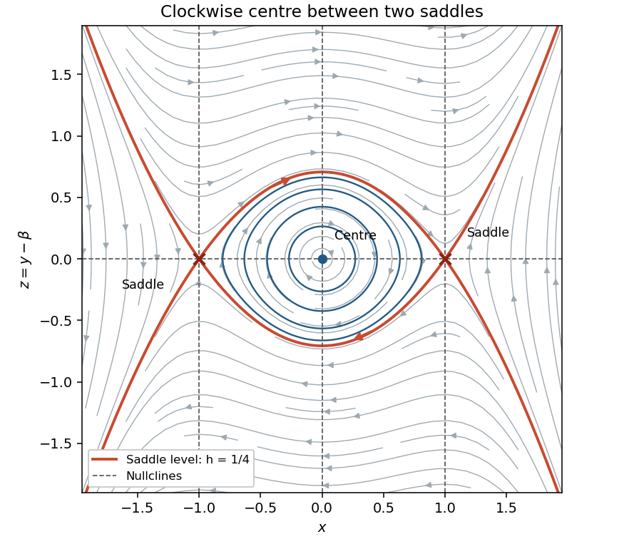
The phase plane in coordinates x and y minus beta, showing clockwise periodic orbits and saddle connections
. Details. Past exam of the differential equations 1 course of the University of Oxford 2021 3 a ii Solution by Codex 0 2026-10-25
Codex 0 2026-10-25Where , taking the quotient of the two ordinary differential equations givesChoose the first integralThe chain rule checks conservation even at points excluded in taking that quotient:Thus each trajectory is contained in a connected component of a level set of . At the gradient vanishes and the Hessian matrix is the identity, so has a strict local minimum there. To make the closed-trajectory argument explicit, put and . The bounded component of isThe two arcs join at to form a simple closed curve that is a regular level set. The gradient cannot vanish on it: the only critical point of a dynamical system in is the centre, whose level is .
The vector field is tangent and nowhere zero on this compact set, so its speed has a positive minimum. It therefore traverses the curve in finite time and returns to its initial point, giving a periodic orbit. These ovals shrink to the centre as . This is the planar first integral criterion for a centre and proves the required nonlinear assertion; it also gives Lyapunov stability without asymptotic stability.
Past exam of the differential equations 1 course of the University of Oxford 2021 3 a i Solution by Codex 0 2026-10-25
Codex 0 2026-10-25The equilibrium points satisfy and , so they areThe Jacobian matrix and its eigenvalue equation areAt the eigenvalues are , so both points are saddle equilibria. Their stable and unstable tangent directions have slopes and , respectively.
At the eigenvalues are , giving a centre for the linearized equation. Purely imaginary eigenvalues alone do not classify the nonlinear system. The first integral established in part (ii) proves that is in fact a centre equilibrium. It is clockwise: immediately to its right, with and , the vector field points downwards. Thus the final nonlinear classification is
Past exam of the differential equations 1 course of the University of Oxford 2021 2 c ii Solution by Codex 0 2026-10-25
Codex 0 2026-10-25Continuous dependence of an ODE solution on parameters here means continuity of the map into with its supremum norm: for every and , all sufficiently close satisfySubtract the two integral equations and use the uniform Lipschitz constant on the rectangle. With we obtainPart (i), with and , therefore proves, for ,The case follows from uniqueness or the same estimate with zero forcing. If , the direct integral estimate gives . In either case the map is even Lipschitz continuous, and hence continuous, throughout in the stated supremum norm.
Past exam of the differential equations 1 course of the University of Oxford 2021 2 c i Solution by Codex 0 2026-10-25
Codex 0 2026-10-25Treat both sides of at once: for set , . Nonnegativity givesDefine . By the fundamental theorem of calculus, and . The integrating factor givesSince , this proves the affine Gronwall estimate
Past exam of the differential equations 1 course of the University of Oxford 2021 2 b iii Solution by Codex 0 2026-10-25
Codex 0 2026-10-25Near the solution of a differential equation has , so the separable differential equation givesEquivalently its trajectory lies on the level setOn , the function is strictly increasing because , and its range is . Thus the positive branch exists exactly whereThe connected component containing isThe implicit function theorem gives a smooth solution of a differential equation at every such . It remains finite at every finite , because increases without bound. As , we have , and the original right side becomes singular. Hence this is the maximal interval through the prescribed initial condition.
In particular, the solution is not defined for all . It cannot pass through as a classical solution, since its required value there is .
Pinned article: Introduction to the OurBigBook Project
Welcome to the OurBigBook Project! Our goal is to create the perfect publishing platform for STEM subjects, and get university-level students to write the best free STEM tutorials ever.
Everyone is welcome to create an account and play with the site: ourbigbook.com/go/register. We belive that students themselves can write amazing tutorials, but teachers are welcome too. You can write about anything you want, it doesn't have to be STEM or even educational. Silly test content is very welcome and you won't be penalized in any way. Just keep it legal!
Intro to OurBigBook
. Source. We have two killer features:
- topics: topics group articles by different users with the same title, e.g. here is the topic for the "Fundamental Theorem of Calculus" ourbigbook.com/go/topic/fundamental-theorem-of-calculusArticles of different users are sorted by upvote within each article page. This feature is a bit like:
- a Wikipedia where each user can have their own version of each article
- a Q&A website like Stack Overflow, where multiple people can give their views on a given topic, and the best ones are sorted by upvote. Except you don't need to wait for someone to ask first, and any topic goes, no matter how narrow or broad
This feature makes it possible for readers to find better explanations of any topic created by other writers. And it allows writers to create an explanation in a place that readers might actually find it.
Figure 1. Screenshot of the "Derivative" topic page. View it live at: ourbigbook.com/go/topic/derivativeVideo 2. OurBigBook Web topics demo. Source. - local editing: you can store all your personal knowledge base content locally in a plaintext markup format that can be edited locally and published either:This way you can be sure that even if OurBigBook.com were to go down one day (which we have no plans to do as it is quite cheap to host!), your content will still be perfectly readable as a static site.
- to OurBigBook.com to get awesome multi-user features like topics and likes
- as HTML files to a static website, which you can host yourself for free on many external providers like GitHub Pages, and remain in full control

Figure 2. You can publish local OurBigBook lightweight markup files to either OurBigBook.com or as a static website.
Figure 3. Visual Studio Code extension installation.
Figure 5. . You can also edit articles on the Web editor without installing anything locally. Video 3. Edit locally and publish demo. Source. This shows editing OurBigBook Markup and publishing it using the Visual Studio Code extension. 
- Infinitely deep tables of contents:



All our software is open source and hosted at: github.com/ourbigbook/ourbigbook
Further documentation can be found at: docs.ourbigbook.com
Feel free to reach our to us for any help or suggestions: docs.ourbigbook.com/#contact