Use the unweighted inner product $⟨w,y⟩={\int }_0^a\overline{w}ydx$. Two applications of integration by parts giveThe given boundary conditions set $y=0$ at both ends, but leave $y^{\prime }(0)$ and $y^{\prime }(a)$ independently variable. The remaining boundary term vanishes for every admissible $y$ precisely when $w(0)=w(a)=0$. Consequently the formal adjoint and the boundary conditions specifying the adjoint operator are

The characteristic equation of the linear ordinary differential equation is $r^2+2r+2=0$, with roots $-1\pm i$. A real pair of homogeneous solutions is thereforeTheir Wronskian, with the convention $W=y_1{y}_2^{\prime }-y_1^{\prime }{y}_2$, isThus the two functions are linearly independent throughout the interval and span its homogeneous solutions.

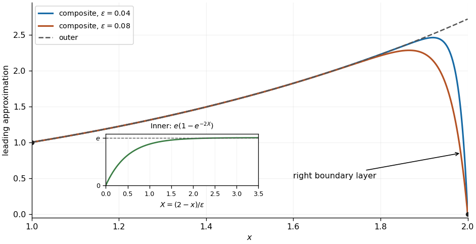
The common value in the overlap region is $e$. The additive composite expansion therefore givesThis leading approximation has $y_{\mathrm{comp},0}(2)=0$ and $y_{\mathrm{comp},0}(1)=1-e^{1-2/ϵ}$; the left endpoint error is exponentially small. It rises from near one following the outer solution $e^{x-1}$, approaches a value close to $e$, then drops rapidly to zero in the right boundary layer. Its first derivative isFor small $ϵ$ the largest value lies slightly inside the interval. For this additive composite expansion, the first derivative vanishes atThis locates the rounded top of the sketch; the rapid final drop has the $O(ϵ)$ scale found above. The additive composite expansion is a leading approximation, so its exponentially small endpoint error does not imply an exponentially small error throughout the interval: neglected algebraic corrections to the outer expansion and inner expansion remain.

The reduced equation and the left boundary condition give the leading outer solutionIntroduce the right inner variable $X=(2-x)/ϵ\ge 0$ and write $Y(X)=y(2-ϵX)$. The chain rule gives $y^{\prime }=-Y_X/ϵ$ and $y^{\prime \prime }=Y_{XX}/{ϵ}^2$. Multiplying the rescaled differential equation by $ϵ$ gives the exact equationAt leading order, $Y_{0,XX}+2Y_{0,X}=0$, with general solution $Y_0=A+B{e}^{-2X}$. The right boundary condition gives $Y_0(0)=0$. The asymptotic matching condition in the overlap region $ϵ\ll 2-x\ll 1$ givesThus $A=e$ and $B=-e$, yielding the leading inner expansionEquivalently, the inner variable $\xi =2(2-x)/ϵ$ gives $Y_0=e(1-e^{-\xi })$. Both normalizations describe the same boundary layer.

Setting $ϵ=0$ gives the reduced first-order linear differential equation $y^{\prime }=y$. Its nonzero solutions cannot satisfy the zero value at $x=2$, so one endpoint needs a boundary layer. To determine which endpoint, freeze the coefficient at $x=x_b>0$ in the rapidly varying part: $ϵy^{\prime \prime }-x_b{y}^{\prime }=0$ has fast mode $e^{x_b(x-x_b)/ϵ}$. It decays into the interval from the right endpoint but grows into the interval from the left endpoint. HenceThe dominant balance $ϵ/{\delta }^2\sim x_b/\delta$ gives $\delta \sim ϵ/x_b$, so a convenient local thickness is $ϵ/2$. The left boundary condition must select the outer solution. Equivalently, a putative left inner variable $X=(x-1)/ϵ$ would give $Y_{XX}-Y_X=0$, whose nonconstant solution grows like $e^X$ and cannot satisfy the asymptotic matching condition as $X\to \infty$.

Putting both data at zero makes this an initial value problem. The uniqueness theorem for ordinary differential equations applies, and one can also prove uniqueness directly: the difference of two solutions is a homogeneous solution $A\cos x+B\sin x$ whose value and first derivative at zero are both zero, forcing $A=B=0$. In fact, for every prescribed continuous function $f$,satisfies both initial data and $y^{\prime \prime }+y=f$. Consequently non-uniqueness is impossible for every $l>0$, including $l=m\pi$. In this setting the kernel is trivial. The boundary conditions at a single endpoint do not give the same self-adjoint operator domain as the two separated Dirichlet boundary conditions, so the earlier exceptional lengths do not apply.

At $l=\pi$, the Fredholm solvability condition isby orthogonality of the Fourier sine basis. Thus a non-unique solution exists exactly when $a=0$, with any real $b$. Since $(d^2/d{x}^2+1)\sin 2x=-3\sin 2x$, the complete family isIf $a\ne 0$ there is no solution, for any $b$. In particular, when $a=b=0$, the family reduces to the kernel $C\sin x$; it is still non-unique. There is no choice of $a,b$ producing a unique solution for this length.

Expand in the Fourier sine basis, using unnormalized eigenfunctions:Projection of $\mathcal{L}y=f$ onto each eigenfunction givesWhen $l\notin \pi {\mathbb{N}}_{>0}$, every eigenvalue is nonzero and the eigenfunction expansion is uniquely determined:When $l=m\pi$, the exceptional index is $n=m$, for which the eigenfunction is $\sin x$. If $f_m\ne 0$, its coefficient equation is $0=f_m$, an inconsistency: there is no solution. If $f_m=0$, the coefficient equation is $0=0$, and $c_m$ is arbitrary. The full family isThis is the Fredholm alternative directly in the coefficient equations: nonzero eigenvalues fix their coefficients; a zero eigenvalue requires zero forcing in that direction and leaves the corresponding coefficient free. An inconsistent equation at a zero eigenvalue cannot be repaired by assigning an infinite coefficient.

For convergence, Lipschitz continuity implies absolute continuity of $f$, with bounded derivative almost everywhere. One integration by parts gives $f_n=O(n^{-1})$; since the denominators grow quadratically, $c_n=O(n^{-3})$ apart from the single free coefficient. The solution series and its first derivative therefore converge uniformly. The second derivative converges in $L^2$, and the resulting Sobolev space solution satisfies $y^{\prime \prime }=f-y$. As $f-y$ is a continuous function, this is a classical $C^2$ solution, with both boundary conditions satisfied. The forcing's Fourier sine series is interpreted on the open interval or in $L^2$; its endpoint values need not equal the endpoint values of $f$.

For $\sin l\ne 0$, use variation of parameters with the homogeneous solutions $\cos x,\sin x$, whose Wronskian is one. Write $y=A(x)\cos x+B(x)\sin x$ and impose $A^{\prime }\cos x+B^{\prime }\sin x=0$. The differential equation gives $-A^{\prime }\sin x+B^{\prime }\cos x=f$, henceAfter integrating from zero and using the left boundary condition,The right boundary condition determinesso the unique solution isCombining the two integrals gives $y(x)={\int }_0^{l}G(x,t)f(t)dt$, with Green's functionIt is symmetric in $x,t$, as expected from self-adjointness, and has zero endpoint values. At $x=t$ it is continuous, while its first derivative obeys the jump conditionThus $({\partial }_x^2+1)G=\delta (x-t)$, with the positive normalization of the Dirac delta function required for $\mathcal{L}y=f$.

The homogeneous solution is $A\cos x+B\sin x$. The left boundary condition removes $A$, and the right boundary condition gives $B\sin l=0$. Thus the kernel of a linear map associated with this boundary value problem isThe Fredholm alternative now gives the complete classification:For necessity at $l=m\pi$, multiply by the homogeneous solution $\sin x$ and use the Lagrange identity for a Sturm-Liouville operator to obtain ${\int }_0^{l}f\sin xdx=0$. For sufficiency, the particular solutionsatisfies $z(0)=0$ and $z^{\prime \prime }+z=f$. At the other endpoint,which is zero under the compatibility condition. All solutions are then $z+B\sin x$, with $B$ arbitrary. The assumed Lipschitz continuity of $f$ in particular makes $f$ continuous, so the displayed integral defines a classical solution. The length $l=0$ is excluded: it would not define a nonempty interval for this boundary value problem.

Take $l>0$ and use the inner product $⟨u,v⟩={\int }_0^l\overline{u}vdx$ on the Hilbert space $L^2(0,l)$. The differential operator has domainwhere $H^2$ is a Sobolev space. Twice applying integration by parts gives the Lagrange identity for a Sturm-Liouville operatorThe Dirichlet boundary conditions make this expression zero for $u,v\in D(\mathcal{L})$, and the formal adjoint is ${\mathcal{L}}^{\ast }=d^2/d{x}^2+1$. To obtain the domain of the adjoint operator, initially impose the boundary conditions only on $u$. The remaining expression is $-[\overline{u^{\prime }}v{]}_0^l$. Since $u^{\prime }(0)$ and $u^{\prime }(l)$ vary independently, it vanishes for all such $u$ exactly when $v(0)=v(l)=0$. The adjoint domain is therefore the original domain: this is full self-adjointness, including the boundary conditions.

Consequently the eigenvalues are real, eigenfunctions for distinct eigenvalues are orthogonal, and regular Sturm-Liouville theory supplies a complete orthonormal eigenbasis. Here these objects can be exhibited explicitly:Indeed $\mathcal{L}{\varphi }_n={\lambda }_n{\varphi }_n$, and the Fourier sine basis is complete in $L^2(0,l)$. There are no additional eigenvalues: for a nonzero eigenfunction $u$, integration by parts givesso $u^{\prime \prime }+(1-\lambda )u=0$ and the endpoint values force $\sqrt{1-\lambda }l=n\pi$. All these eigenvalues are simple. The eigenvectors are precisely the nonzero multiples of these eigenfunctions, regarded as vectors in the Hilbert space.

Choose the real leading eigenfunction $y_1=C\sin x$, keeping its amplitude $C\ne 0$ fixed. At first order in the regular perturbation expansion, the equation becomesThe operator $L=D^2+1$ with these homogeneous Dirichlet boundary conditions is self-adjoint, as allowed in the question, and its null space is spanned by $y_1$. The Fredholm solvability condition requires the forcing to be orthogonal to that null space:The same condition follows directly by integrating $y_{1}L{y}_{11}$ by parts: the endpoint term $[y_1{y}_{11}^{\prime }-y_1^{\prime }{y}_{11}{]}_0^{\pi }$ vanishes, and $L{y}_1=0$. Since a nonzero real $y_1$ has a positive squared integral,This is the requested expression and is an instance of the leading nonlinear eigenvalue shift in a Sturm-Liouville problem. In the amplitude convention above, ${\int }_0^{\pi }{\sin }^{2}xdx=\pi /2$ and ${\int }_0^{\pi }{\sin }^{3}xdx=4/3$, so ${\lambda }_{11}=-8C/(3\pi )$. For the particular choice $C=1$, it is $-8/(3\pi )$.

The amplitude dependence of a nonlinear eigenvalue correction follows here from the quadratic term: rescaling the eigenfunction changes the eigenvalue shift. There is no single numerical correction independent of the chosen leading amplitude. Once the solvability condition is met, $y_{11}$ is determined up to addition of a multiple of $y_1$; a normalization such as ${\int }_0^{\pi }{y}_1{y}_{11}dx=0$ can fix that remaining freedom.

For a positive eigenvalue write $\mu =\sqrt{\lambda }>0$. The general solution of the limiting constant-coefficient differential equation is $y=A\cos (\mu x)+B\sin (\mu x)$. The endpoint at zero gives $A=0$. A nonzero eigenfunction then requires $B\ne 0$, and the endpoint at $\pi$ gives $\sin (\mu \pi )=0$. ConsequentlyFor real eigenfunctions the constants may be any nonzero real amplitudes. Requiring unit L2 norm would set $|C_k|=\sqrt{2/\pi }$, but that normalization is not required by the question. The lowest eigenvalue is ${\lambda }_1=1$ and its eigenspace is spanned by $\sin x$. For completeness, zero yields only an affine solution annihilated by both endpoints, and negative eigenvalues yield hyperbolic functions whose two zero endpoint values also force the zero solution.

For every real $r$ and integer $n\ge 1$, $|\sin r|\le \min (1,|r|)$ givesThis estimate covers both even and odd $n$, without any assumption on the sign of $u$. Since $a(t)\ge 0$, the energy estimate from part (i) becomesEquivalently, an integrating factor givesThe bracket is nonnegative and starts at zero, so it vanishes identically. This is also the zero-data case of the Gronwall inequality. The vanishing L2 norm and continuity of $u$ imply

Define the squared L2 norm $E(t)={\int }_0^{1}u(x,t{)}^{2}dx$. Multiplication of the semilinear partial differential equation by $u$, followed by integration by parts, givesAt $x=1$ the Dirichlet boundary condition makes the boundary term zero. At $x=0$ the Robin boundary condition is $u_x(0,t)=\alpha u(0,t)$, so subtraction of the lower endpoint gives $-\alpha u(0,t{)}^2$. In particular the sign is dissipative. Thus the exact energy identity iswhich implies

The parabolic boundary values are zero. An exact solution satisfies the preceding differential inequality, so its maximum estimate with $A=0$ gives $u\le 0$. The function $v=-u$ satisfies the same equation because both the linear differential operator and the cubic term change sign. Applying the same maximum principle to $v$ gives $-u\le 0$. Hence the complete solution set isSubstitution verifies existence, and the two inequalities prove uniqueness among the assumed smooth solutions for every continuous choice of the drift coefficients.

With zero drift, choose the smooth functionIt equals $-1$ on the entire parabolic boundary, so $A=-1$. On the closed cylinder, $-1\le u\le -7/8$, whileConsequentlyNevertheless the maximum at $(0,0,1)$ isThe negative cubic term permits an interior increase while the boundary stays fixed, explaining why the sign condition in the preceding part matters.

Let $\mathcal{P}u=u_t-\Delta u+a{u}_x+b{u}_y$ on the unit disk over $0<t\le 1$. Smoothness is understood to include continuity on the closed cylinder. If $u$ exceeded its nonnegative parabolic boundary maximum $A$, it would attain a positive global maximum $M>A$ at some spatial interior point at time $t_0>0$. There,At $t_0=1$ the last inequality uses the derivative from the past; at an interior time it is equality. These signs imply $\mathcal{P}u+u^3\ge M^3>0$, contradicting the given differential inequality. ThusIf $A>0$, equality at any point of $Q$ gives the same contradiction with $M=A$, so $u<A$ throughout $Q$. If $A=0$, equality is possible: $u\equiv 0$ is an example. More precisely, write the inequality as $\mathcal{P}u+cu\le 0$ with $c=u^2\ge 0$. The strong parabolic maximum principle shows that an interior zero at time $t_0>0$ forces $u\equiv 0$ on $B\times [0,t_0]$.

That conclusion need not extend into the future for a subsolution. For $t_0<1$, take a spatially constant function which is zero for $t\le t_0$ and equals $-\exp (-1/(t-t_0))$ for $t>t_0$. It is smooth, nonincreasing and nonpositive, so $\mathcal{P}u+u^3\le 0$, but it becomes negative after $t_0$.

Use the compatible open semicircles and set $r=\sqrt{x^2+y^2}$. The characteristic curve through $(\cos \theta ,\sin \theta ,-1)$ hasThe condition $s<1$ is essential: at $s=1$ there is finite-time blowup, so the opposite branch cannot be reached from the data. From $r=(1-s\sin \theta {)}^{-1}$ and $y=r\sin \theta$,Eliminating $s$ yieldsThe ratio inside the cube root is positive precisely on the two data-determined regionsOn $D_{+}$ each point traces to the upper semicircle, and on $D_{-}$ to the lower semicircle, with $s<1$. To check the parameter ranges explicitly, for $\eta =\sin \theta >0$ they are $-\infty <s<1$, whereas for $\eta <0$ they are $1/\eta <s<1$. At the latter lower endpoint the planar projection escapes to infinity. The inverse function theorem and uniqueness for the characteristic ordinary differential equations give a unique smooth solution on each region. Equivalently, each point has the unique foot $(x/r,y/r)$ and parameter $(r-1)/y$.

A direct check is particularly short. For $s=(r-1)/y$, let $\mathcal{D}=xy{\partial }_x+y^2{\partial }_y$. Then $\mathcal{D}r=yr$, $\mathcal{D}y=y^2$, andSince $dz/ds=-z^4/3$, the displayed formula solves the partial differential equation, and $r=1$ gives $z=-1$ on both open semicircles. The finite boundary where $r=1+y$, away from the axis, is the parabola $y=(x^2-1)/2$ and corresponds to blowup. Points on $y=0$ cannot be added to a classical continuation of these regions: where they are approached from a data-determined region, the height behaves like a nonzero multiple of $|y{|}^{1/3}$, or has incompatible limits at the endpoints. The formula is therefore the complete classical answer for the compatible arcs, while the full-circle problem as printed has no classical solution.

Parametrize the data by $(\xi ,\eta ,\zeta )=(\cos \theta ,\sin \theta ,-1)$. The determinant testing Noncharacteristic Cauchy data isThus the open upper and lower semicircles are noncharacteristic, but the entire circle is not a valid noncharacteristic data curve: the determinant vanishes at $(1,0)$ and $(-1,0)$.

There is a stronger obstruction at those two points. On $y=0$, the differential equation forces $0=-z^4/3$, and hence $z=0$. This contradicts the prescribed value $z=-1$ at both endpoints. ThereforeThe obstruction is already present if the equation is imposed next to the circle and the solution and its first partial derivatives extend continuously to it.

Away from the endpoints, the characteristic projections are radial half-lines:For $\sin \theta >0$, $r$ increases with $s$; for $\sin \theta <0$, $r$ decreases with $s$. Each projection meets its own open semicircle exactly once and never crosses $y=0$. The endpoint projections themselves are single stationary points, although their lifted characteristic curves have varying height.