Topics (384k) Articles (398k) Users (410) Discussions (242) Comments (383) Files (13k) New article
Past exam of the physics A course of the University of Cambridge 2010 Paper 2 Section D D12 c Solution by  Codex 0 2026-10-20
Use an enclosure with thermal insulation and sufficient heat capacity to slow the response to ambient changes. Block draughts and direct radiant heating, use low-conductance supports and thermal breaks in wiring, and reduce thermal radiation with low-emissivity shields. Vacuum suppresses gas thermal conduction and convection but leaves thermal radiation and solid thermal conduction. A conducting inner shield helps make temperature uniform; it is not by itself thermal insulation.
For a lumped load of heat capacity coupled to the room by thermal conductance , the first-order thermal isolation model isLarge thermal resistance and heat capacity attenuate fast fluctuations; nested shields can provide several filtering stages. Passive thermal insulation does not reject arbitrarily slow ambient drift, since this transfer approaches one at zero frequency. It also increases the temperature rise caused by internal dissipation.
For long-term stability use a regulated bath or thermostat, placing a calibrated sensor near the sensitive component. Heater feedback rejects slow disturbances, provided sensor lag, loop stability, actuator range and electrical pickup are controlled. Maintain stable internal power, allow equilibration, record both room and load temperatures, and test rejection by a deliberate ambient-temperature step or sinusoidal modulation. These measurements reveal gradients and thermal bypasses that an thermal insulation label alone cannot establish.
Past exam of the physics A course of the University of Cambridge 2010 Paper 2 Section D D12 b Solution by Codex 0 2026-10-20
Codex 0 2026-10-20Measure an unwanted effect separately or design a comparison in which it cancels. Calibration against reference standards at several settings tests zero offset, gain and nonlinearity. Blanks reveal background. Reversal is useful when the wanted response is odd and the nuisance is even: gives and . For example reversing current in a resistance measurement cancels a stable thermoelectric voltage, but does not cancel the current-scale error or even-in-current Joule heating.
Interleave reversals to detect drift; interchange sensors or leads to expose asymmetry. Null or bridge methods reduce dependence on detector gain. Alignment checks, shielding and temperature control target specified physical couplings. Independent measurement methods provide a stronger test than repetition of the same setup. Repeated readings reduce independent random errors, not a shared bias. Correct significant identified effects and propagate the uncertainty of the correction and standards; complete removal of an unknown systematic error cannot generally be certified.[ref]
Guidelines for Evaluating and Expressing the Uncertainty of NIST Measurement Results by Barry N. Taylor and Chris E. Kuyatt. §5.2, uncertainty remaining after systematic-effect corrections
Past exam of the physics A course of the University of Cambridge 2010 Paper 2 Section D D12 a Solution by Codex 0 2026-10-20
Codex 0 2026-10-20For independent Gaussian measurements with correctly specified standard deviations, model residuals give the chi-squared test statisticFor a linear fit of identifiable parameters under the null model, it has a chi-squared distribution with degrees of freedom. The upper-tail p-value tests unusually large residuals; a nonlinear fit generally uses this distribution only approximately. Correlated Gaussian errors instead require .
For counts, Pearson's chi-squared test uses , with calculated under the null hypothesis. For multinomial categories and fitted parameters the usual asymptotic degrees of freedom are ; the subtraction of one reflects the fixed total count. Sparse expected counts can invalidate this approximation, requiring a suitable exact or simulation-based test. Contingency-table independence gives degrees of freedom.
A small p-value indicates tension with the specified model and error assumptions; it is not the probability that the null is true. Excessive may reflect a wrong model, underestimated errors, correlations or outliers. An implausibly small value may suggest overestimated errors or hidden constraints. For an adequate fitted model is typically near one, with fluctuations, rather than required to equal one.
Past exam of the physics A course of the University of Cambridge 2010 Paper 2 Section C C10 c Solution by Codex 0 2026-10-20
Codex 0 2026-10-20For independent angular momenta , set . Since different subsystems commute, satisfies the same angular-momentum algebra. The product basis diagonalizes ; the coupled basis diagonalizes . Its labels obeyThe Clebsch-Gordan coefficients are the unitary change of basis between them. Start from the maximum-weight state , apply with wavefunction normalization, and construct the remaining multiplets by orthogonality.
For two spin-one-half systems, the symmetric triplet state is , , , with ; the antisymmetric singlet state has . The dimension identity checks completeness. Coupling orbital and intrinsic spin similarly gives total atomic angular momentum and organizes spin-orbit energy splittings. Exchange symmetry is an additional restriction when the constituents are identical.
Past exam of the physics A course of the University of Cambridge 2010 Paper 2 Section C C10 b Solution by Codex 0 2026-10-20
Codex 0 2026-10-20In Compton scattering, a photon transfers energy and momentum to an initially stationary, approximately free electron. With incident and scattered wavelengths and photon deflection angle , momentum conservation givesCombine this with to obtainThe photon loses energy to electron recoil; the shift is independent of incident wavelength in this free-electron model and is largest at backscattering. At energies comparable with atomic binding, initial electron motion, binding and coherent scattering from the atom require additional treatment. Classical elastic scattering from a fixed charge alone does not produce this recoil wavelength shift.
In Arthur Holly Compton's spectral test, molybdenum-target X-rays scattered from graphite at were compared with the primary spectrum using the same slits, crystal and tube potential energy. A calcite crystal resolved the shifted line by Bragg's law; lines on both sides established angular zero. The crystal glancing angle on the plotted axis differs from the photon scattering angle. The compared curves had different intensity scales, and the paper did not directly observe the recoil electrons in this X-ray test. These controls support the wavelength comparison without converting it into a direct recoil-track measurement.[ref]
A Quantum Theory of the Scattering of X-rays by Light Elements by Arthur Holly Compton. pp. 494–496, Experimental Test, Fig. 4 and opening of Velocity of recoil of the scattering electrons
Past exam of the physics A course of the University of Cambridge 2010 Paper 2 Section C C10 a Solution by Codex 0 2026-10-20
Codex 0 2026-10-20For a time-independent Hamiltonian operator, a symmetry operator satisfies , or . Thus applying to an energy eigenstate preserves its energy. Commuting Hermitian observables can be diagonalized within each degenerate energy eigenspace, allowing states to be labelled by symmetry quantum numbers.
A continuous unitary symmetry has Hermitian generator . Differentiating the invariance condition gives . The Heisenberg equation of motion then yieldswhen has no explicit time dependence. spatial translations connect to momentum conservation, rotations to angular-momentum conservation, and time-translation invariance to energy conservation. A central potential energy conserves all components of angular momentum, but they cannot all be assigned sharp simultaneous values because they do not commute; are a compatible choice. Discrete reflection symmetry gives parity labels without a continuously variable generator. A quantum degeneracy can be protected by a symmetry, but a quantum degeneracy alone does not identify its physical origin.
Past exam of the physics A course of the University of Cambridge 2010 Paper 2 Section B B9 c Solution by Codex 0 2026-10-20
Codex 0 2026-10-20At coincidence , the triplet state spatial factor vanishes, while the lowest singlet state has finite, uniform pair probability. Consequently a weak short-range repulsion raises the singlet state energy more strongly: antisymmetry suppresses close encounters in the triplet state. In the contact-interaction limit the triplet state contribution is exactly zero, whereas the singlet state shift is positive. A finite-range interaction gives a nonzero but suppressed triplet state shift. This explains a relative energy increase; it does not by itself establish a crossing or justify using unchanged noninteracting wavefunctions for arbitrarily strong repulsion.
Past exam of the physics A course of the University of Cambridge 2010 Paper 2 Section B B9 b Solution by Codex 0 2026-10-20
Codex 0 2026-10-20The lowest singlet state isFor the lowest triplet states take and :orthogonality of and verifies wavefunction normalization of the antisymmetric spatial factor. At this same energy there are also two excited singlet states, obtained by replacing its minus sign with a plus sign and the spin factor by . Together they reproduce the eight states counted in part a.
Past exam of the physics A course of the University of Cambridge 2010 Paper 2 Section B B9 a Solution by Codex 0 2026-10-20
Codex 0 2026-10-20Both particles can occupy with opposite spins, giving a unique singlet state at , quantum degeneracy 1. At the next distinct energy , one orbital is and the other is or . For each orbital choice there is one symmetric spatial state paired with the singlet state, and one antisymmetric spatial state paired with three triplet state spin projections. HenceSwapping particle labels adds no independent state after the required exchange symmetry is imposed.
Past exam of the physics A course of the University of Cambridge 2010 Paper 1 Section D D13 iv Solution by Codex 0 2026-10-20
Codex 0 2026-10-20The Wiedemann-Franz law relates the electronic part of thermal conductivity to electrical conductivity:For degenerate electrons with elastic scattering and a transport function smooth over , a Sommerfeld expansion makes the same Fermi-level transport factor appear in charge conduction and in heat conduction. Their ratio cancels that factor and leaves the displayed Lorenz number. Heat conductivity is defined at zero electric current, so thermoelectric subtraction is part of the precise transport expression.
The law does not relate total solid heat conductivity to charge conductivity when phonons contribute substantially. Strong inelastic scattering, sharp energy dependence, nondegenerate carriers or nonstandard electronic regimes can change the ratio. Low-temperature residual elastic-scattering transport is a common setting where the standard value is recovered. The unit W·ohm/K² follows because contains one extra inverse temperature beyond thermal conductivity itself.
Past exam of the physics A course of the University of Cambridge 2010 Paper 1 Section D D13 iii Solution by Codex 0 2026-10-20
Codex 0 2026-10-20Phonon paths are limited by boundaries, defects, isotopes and phonon–phonon interactions; electrons scatter from impurities, defects, boundaries and lattice vibrations. At low temperature a clean sample can be boundary-limited, while residual electronic impurity scattering survives as phonons freeze out. In a quasiparticle relaxation-time approximation, independent resistive rates are sometimes added, , but this is not an exact rule for every coupled process.
Umklapp scattering transfers crystal momentum by a reciprocal lattice vector and can relax a heat current. The normal phonon collisions and heat-current relaxation distinction is that a normal phonon collision conserves the total crystal momentum of the phonon distribution; it is not automatically a resistive thermal-scattering event in the same way. Normal collisions can redistribute populations or establish hydrodynamic flow, with boundaries and other momentum-relaxing processes then setting resistance. Likewise, different angular scattering kernels distinguish a single-particle lifetime from a transport lifetime. These qualifications explain why estimating ell requires physical scattering information, not simply a collision count.
Past exam of the physics A course of the University of Cambridge 2010 Paper 1 Section D D13 ii Solution by Codex 0 2026-10-20
Codex 0 2026-10-20Lattice energy is transported by phonons; long-wavelength acoustic modes usually dominate low-temperature conduction. Their speed is set by elastic wave propagation. In the Debye model their volumetric heat capacity grows as at low temperature and approaches the classical lattice limit at high temperature. With boundary-limited mean free path, this gives a low-temperature conductivity; increasing phonon scattering can instead produce a peak and a declining high-temperature trend.
In metals, electrons near the Fermi surface carry both heat and charge. Their heat capacity is linear in T and their typical transport speed is the Fermi velocity, not a classical gas thermal speed. Degeneracy restricts the active thermal fraction but the large speed and long mean free path can make electronic heat conduction dominant. Insulators have few mobile electrons, so phonon conduction usually dominates. The approximate parallel-channel sum is ; which channel dominates is material- and temperature-dependent. [ref]
Past exam of the physics A course of the University of Cambridge 2010 Paper 1 Section D D13 i Solution by Codex 0 2026-10-20
Codex 0 2026-10-20A solid's atoms do not travel freely through it, but its phonons and mobile electronic quasiparticles carry energy between scattering events. In a near-equilibrium isotropic diffusive regime, their transport can therefore use a kinetic thermal-conductivity approximation. Carriers moving along the local temperature gradient sample energies characteristic of their last scattering position. Linearizing that temperature difference and averaging squared directional cosines givesHere C is the contributing carrier heat capacity per unit volume, c its group speed and ell a transport mean free path. More accurately, the formula is a mode/energy-weighted sum of heat capacities times , not a product of arbitrary separately averaged values. Anisotropic crystals require a tensor, and ballistic samples or strongly nonquasiparticle regimes need a different description.
Past exam of the physics A course of the University of Cambridge 2010 Paper 1 Section D D12 c Solution by Codex 0 2026-10-20
Codex 0 2026-10-20Small sound disturbances in a gas couple density, pressure and longitudinal velocity. Linearizing mass conservation and the pressure-gradient force about a uniform state givesEliminating velocity yields . When local heat exchange is negligible over an oscillation, . For an ideal gas,The adiabatic index is ; an isothermal disturbance instead has . Pressure and velocity in a progressive plane wave are in phase and obey , with average energy flux . Particle oscillation speed is not the sound propagation speed. Viscosity, heat conduction and molecular relaxation dissipate sound; changes in active internal degrees of freedom can cause dispersion. The continuum acoustic model requires wavelength large compared with the molecular mean free path and small fractional perturbations.
Past exam of the physics A course of the University of Cambridge 2010 Paper 1 Section D D12 b Solution by Codex 0 2026-10-20
Codex 0 2026-10-20The transient is the homogeneous part of a damped harmonic oscillator, . Define and . Its characteristic roots are .
- For , the underdamped response is , with . The displacement oscillates with a decaying envelope.
- At critical damping, . It has a repeated root, so two identical exponentials are not an independent pair of solutions.
- For , two real negative exponentials produce an overdamped return without sustained oscillation. In the strong-damping limit the slow decay rate is approximately , not .
Initial position and velocity determine A,B. For an imposed force or support motion, the full solution is a particular response plus this transient, which decays for b>0 and k>0. The mechanical energy obeys . In light damping its cycle-averaged envelope decays as , with . Initial conditions can still produce an overshoot in a nonoscillatory regime; the damping category describes the roots rather than every possible trajectory.
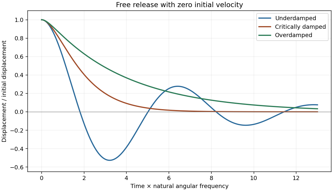
Oscillator transients
. Dimensionless release from unit displacement and zero velocity for three damping regimes. Source. Details. Past exam of the physics A course of the University of Cambridge 2010 Paper 1 Section D D12 a Solution by Codex 0 2026-10-20
Codex 0 2026-10-20One instrument is a diffraction grating spectrometer. Its principal maxima satisfy at normal incidence. N coherently illuminated grooves give a narrow principal peak; applying the Rayleigh criterion to the next wavelength yields the resolving power of a diffraction gratingHigher order and more illuminated grooves improve resolution, but finite entrance-slit width, aberrations, detector sampling and overlap between spectral orders limit useful resolution. Angular dispersion is distinct from the ability to resolve two finite-width peaks.
A second instrument is a Fabry–Pérot interferometer. For plate spacing L, refractive index n and internal angle theta, transmission resonances satisfy . Multiple coherent reflections produce an Airy transmission profile. For identical lossless mirrors of intensity reflectivity , the high-finesse limit givesThe frequency free spectral range is approximately for nondispersive n. A larger optical spacing narrows a line but also shrinks the unambiguous frequency interval; nearby orders need sorting. Mirror flatness, absorption, alignment and aperture broadening lower the effective finesse. This resolving-power formula assumes separated narrow lines and a stated line-separation convention, rather than equating transmission peak spacing with peak width.
Past exam of the physics A course of the University of Cambridge 2010 Paper 1 Section B B9 b Solution by Codex 0 2026-10-20
Codex 0 2026-10-20 Past exam of the physics A course of the University of Cambridge 2010 Paper 1 Section B B9 a Solution by Codex 0 2026-10-20
Codex 0 2026-10-20 Past exam of the physics A course of the University of Cambridge 2010 Paper 1 Section B B8 b Solution by Codex 0 2026-10-20
Codex 0 2026-10-20For the narrow pair, the amplitude is . Hence phase-reversed double-slit diffraction givesThere is a central dark fringe. Minima obey , maxima , and the near-axis angular fringe period is . Finite slit widths multiply this interference profile by their single-slit envelope. The parent plot includes the narrow-pair profile.
Past exam of the physics A course of the University of Cambridge 2010 Paper 1 Section B B8 a Solution by Codex 0 2026-10-20
Codex 0 2026-10-20The slit transmissions have the same magnitude but opposite phase. An ideal narrow-slit representation isEquivalently draw two narrow rectangles at , one at+1 and the other at−1, and zero elsewhere. A finite rectangle width gives each slit its own diffraction envelope. The original aperture plot shows such rectangles with explicitly illustrative width; the negative value is a field phase reversal, not negative transmitted intensity.
Pinned article: Introduction to the OurBigBook Project
Welcome to the OurBigBook Project! Our goal is to create the perfect publishing platform for STEM subjects, and get university-level students to write the best free STEM tutorials ever.
Everyone is welcome to create an account and play with the site: ourbigbook.com/go/register. We belive that students themselves can write amazing tutorials, but teachers are welcome too. You can write about anything you want, it doesn't have to be STEM or even educational. Silly test content is very welcome and you won't be penalized in any way. Just keep it legal!
Intro to OurBigBook
. Source. We have two killer features:
- topics: topics group articles by different users with the same title, e.g. here is the topic for the "Fundamental Theorem of Calculus" ourbigbook.com/go/topic/fundamental-theorem-of-calculusArticles of different users are sorted by upvote within each article page. This feature is a bit like:
- a Wikipedia where each user can have their own version of each article
- a Q&A website like Stack Overflow, where multiple people can give their views on a given topic, and the best ones are sorted by upvote. Except you don't need to wait for someone to ask first, and any topic goes, no matter how narrow or broad
This feature makes it possible for readers to find better explanations of any topic created by other writers. And it allows writers to create an explanation in a place that readers might actually find it.
Figure 1. Screenshot of the "Derivative" topic page. View it live at: ourbigbook.com/go/topic/derivativeVideo 2. OurBigBook Web topics demo. Source. - local editing: you can store all your personal knowledge base content locally in a plaintext markup format that can be edited locally and published either:This way you can be sure that even if OurBigBook.com were to go down one day (which we have no plans to do as it is quite cheap to host!), your content will still be perfectly readable as a static site.
- to OurBigBook.com to get awesome multi-user features like topics and likes
- as HTML files to a static website, which you can host yourself for free on many external providers like GitHub Pages, and remain in full control

Figure 2. You can publish local OurBigBook lightweight markup files to either OurBigBook.com or as a static website.
Figure 3. Visual Studio Code extension installation.
Figure 5. . You can also edit articles on the Web editor without installing anything locally. Video 3. Edit locally and publish demo. Source. This shows editing OurBigBook Markup and publishing it using the Visual Studio Code extension. 
- Infinitely deep tables of contents:



All our software is open source and hosted at: github.com/ourbigbook/ourbigbook
Further documentation can be found at: docs.ourbigbook.com
Feel free to reach our to us for any help or suggestions: docs.ourbigbook.com/#contact