Topics (384k) Articles (398k) Users (410) Discussions (242) Comments (383) Files (13k) New article
Past exam of the physics B course of the University of Cambridge 2011 Paper 2 Section B B6 i Solution by  Codex 0 2026-10-20
For the dielectric half-space the two formal sources coincide at , outside the region being represented. Their sum is in the dielectric Coulomb kernel, henceThere is no charge singularity inside this half-space. The expression satisfies Laplace's equation there, decays at infinity, and matches the vacuum solution's tangential electric field and normal electric displacement. The coincident image is a mathematical representation, not an extra physical charge in the vacuum region.
Past exam of the physics B course of the University of Cambridge 2011 Paper 1 Section B B8 d Solution by Codex 0 2026-10-20
Codex 0 2026-10-20A rapidly spinning gyroscope approximately has angular momentum along its axle. With no torque in an inertial frame, this vector retains its direction. A transverse torque changes its direction according to ; it does not initially push the axle in the direction of the applied force.
For a fixed pivot, centre of mass from it and gravity , the torque is . In slow steady precession about the vertical, , givingThe factor appears both in torque and in the radius traced by the angular-momentum tip, so it cancels for a nonvertical axle. Reversing spin reverses this precession. The full symmetric-top steady condition is ; the approximation neglects its quadratic term. Sudden release can also produce nutation, so large spin alone does not guarantee a steady sweep.
A wheel-on-pivot experiment can compare precession periods at different measured spin speeds and reverse the spin. Keep the pivot and centre of mass fixed; bearing friction, spin decay, an initial push and support motion can mimic departures from the predicted inverse-spin relation. A freely gimballed direction reference and a gravity-loaded precessing wheel test different torque conditions.[ref]
Past exam of the physics B course of the University of Cambridge 2011 Paper 1 Section B B8 c Solution by Codex 0 2026-10-20
Codex 0 2026-10-20A tidal force measures the difference of gravitational acceleration across an extended object. A freely falling reference frame removes a spatially uniform acceleration, but not its gradient. For a distant point mass at distance and direction from the reference centre, a small internal displacement givesThe tidal tensor has eigenvalues radially and in each transverse direction: radial stretching and transverse squeezing. Its trace vanishes in the source-free region, consistent with the gravitational Gauss law. An associated relative potential is .
The scale is across size , not the centre's absolute gravity . This distinction explains how a more distant massive object can exert a large force but a modest tide. Opposite-side stretching supports the elementary two-bulge picture; real ocean tides also involve rotation, basin geometry and fluid dynamics, so the static gradient alone does not predict coastal heights or timing. The same gradient stresses satellites and can disrupt a self-gravitating body when it competes with the body's own gravitational restoring acceleration.
Past exam of the physics B course of the University of Cambridge 2011 Paper 1 Section B B8 b Solution by Codex 0 2026-10-20
Codex 0 2026-10-20Kepler's laws of planetary motion state that, in the relative two-body description, bound trajectories are ellipses with the attracting body at a focus, the radius vector sweeps equal areas in equal times, and the square of the period is proportional to the cube of the semimajor axis for a fixed total mass. Their Newtonian derivation is especially informative. With relative coordinate and , the inverse-square acceleration is . Its zero torque conserves , fixing a plane and the areal velocity .
For , the orbit equation is as a function of polar angle. ThereforeBound negative-energy motion has and semilatus rectum . Dividing ellipse area by areal velocity givesFor a planet much lighter than its star, replace by . Zero-energy and positive-energy encounters are parabolic and hyperbolic rather than periodic ellipses. Perturbations from other bodies and departures from point-mass Newtonian gravity can precess or otherwise modify the orbit; Kepler's laws are a two-body approximation, not an exact rule for every observed planetary path.
Past exam of the physics B course of the University of Cambridge 2011 Paper 1 Section B B8 a Solution by Codex 0 2026-10-20
Codex 0 2026-10-20A galilean transformation relates inertial frames in uniform relative translation. For the velocity of the primed origin,Absolute time and invariant acceleration make Newton's second law retain its form for the usual nonrelativistic interactions. For a particle of mass , and . Momentum and kinetic energy are frame dependent, although an isolated system's conservation laws hold in either inertial frame. Relative velocities and collision predictions are consistent between frames. A rotating or accelerating frame instead requires inertial-force terms. Maxwell equations with a fixed light speed are not Galilean invariant; Lorentz transformations replace these relations when relativistic effects matter.
Past exam of the physics B course of the University of Cambridge 2011 Paper 1 Section B B6 d Solution by Codex 0 2026-10-20
Codex 0 2026-10-20In charge- and current-free vacuum, Maxwell equations reduce toTaking a curl and using givesand the same wave equation for . For a plane wave , , and . Thus the fields are transverse, mutually perpendicular and in phase; polarization describes the electric-field trajectory at a fixed point.
The energy density and Poynting vector areFor a linearly polarized sinusoid with peak electric amplitude , the mean intensity is . Electromagnetic momentum density is ; normal absorption produces radiation pressure , while ideal retroreflection doubles it. Linear superposition permits interference and standing waves, whose local electric and magnetic fields need not have the traveling-plane-wave equality point by point.
Past exam of the physics B course of the University of Cambridge 2011 Paper 1 Section B B6 c Solution by Codex 0 2026-10-20
Codex 0 2026-10-20For a fixed circuit, Faraday's law of induction readsSurface orientation and contour direction obey the right-hand rule. The negative sign is Lenz's law: a passive induced current acts against the flux change, consistently with energy conservation. The induced electric field generally has nonzero curl and cannot be represented by one single-valued electrostatic potential.
For a material circuit moving with local velocity , the measured electromotive force includes the magnetic Lorentz force on its carriers:This distinguishes transformer induction in a stationary coil from motional induction in a changing circuit. A straight sliding rod of length moving perpendicular to itself and to uniform has . With circuit resistance , the electrical power equals the external mechanical power needed to oppose magnetic drag. An ideal transformer gives in magnitude from common flux linkage; real leakage, resistance and core losses limit that simple result. pickup coils measure flux change rather than an absolute static magnetic field, so integration and a reference state are needed to recover a field history.
Past exam of the physics B course of the University of Cambridge 2011 Paper 1 Section B B6 b Solution by Codex 0 2026-10-20
Codex 0 2026-10-20An electric dipole has equal and opposite charges separated by a small vector from negative to positive, with electric dipole moment . More generally, a localized neutral distribution has , independent of origin. At distances large compared with its size, the leading nonzero term in the multipole expansion isThe field points along on either axial side and opposite in the equatorial plane; its axial magnitude is twice the equatorial magnitude at equal radius. Near the charges the finite-charge expression must replace the far-field approximation.
A permanent dipole in an externally imposed slowly varying electrostatic field has interaction energy , torque and force for fixed . A uniform field aligns it but gives no net force. For a linearly induced dipole , the formation-inclusive energy is , not : the moment itself grows while the field is applied. Dipole density gives electric polarization, whose bound charges are and .
Past exam of the physics B course of the University of Cambridge 2011 Paper 1 Section B B6 a Solution by Codex 0 2026-10-20
Codex 0 2026-10-20Gauss's law connects electric flux through a closed surface to its enclosed charge:The differential form follows from the divergence theorem. The law is exact; extracting a field magnitude by simple division additionally needs symmetry. For spherical symmetry, ; a uniformly charged ball therefore has a field linear in inside and an inverse-square field outside. An infinite line of linear charge density gives by a cylindrical surface. A uniformly charged infinite sheet gives on either side by a pillbox.
An electrostatic conductor has zero interior field and constant potential; excess charge occupies its surface. A pillbox gives when the inside is conducting. More generally, . For dielectric matter, separates bound polarization charge from free charge. Gauss's law alone does not establish a uniform field for an arbitrary finite plate or recover a detailed nonsymmetric charge distribution from one flux measurement.
Past exam of the physics B course of the University of Cambridge 2010 Paper 2A Section D D17 d Solution by Codex 0 2026-10-20
Codex 0 2026-10-20Orthogonality means zero inner product, not merely that two objects look different. For complex vectors, ; for functions a common choice is with positive weight . An orthonormal set has .
For an orthogonal set, the component of along has coefficientA complete orthonormal set gives in the appropriate norm and Parseval's identity . Without completeness there can be a nonzero residual orthogonal to the entire chosen set. Orthogonal nonzero vectors are linearly independent, but independence alone does not imply orthogonality.
Fourier coefficients are projections becauseLikewise, for a self-adjoint operator, gives , so distinct eigenvalues have orthogonal eigenvectors. Degeneracy does not itself force a chosen pair to be orthogonal, but an orthonormal basis can be selected within each eigenspace. The differential version uses the correct Sturm-Liouville weight and boundary conditions.
For mechanical normal modes with unequal masses the relevant inner product is . This makes the modes in D14 orthogonal even when an ordinary unweighted dot product does not. Expanding in such coordinates diagonalizes the kinetic and potential quadratic forms, explaining why modal motions evolve independently and their energies add.
Past exam of the physics B course of the University of Cambridge 2010 Paper 2A Section D D17 c Solution by Codex 0 2026-10-20
Codex 0 2026-10-20Convolution describes the response of a linear time-invariant system to an arbitrary input. If is its impulse response and its input,This is a weighted sum of responses to shifted impulses. For integrable functions the operation is commutative and associative. A causal system has for , restricting the integral to past inputs. With the Fourier convention , the convolution theorem gives .
For example, an RC low-pass frequency response has and , where is the Heaviside step function. Fast input variations are smoothed. The same mathematics describes optical blurring by a point spread function and many other linear response measurements.
Deconvolution tries to recover from measured and known . In noise-free data one formally sets where . Zeros of lose corresponding information; small values amplify measurement noise. If the measured spectrum is , the direct estimate has error , which can be very large at frequencies strongly suppressed by the instrument. An inverse is therefore not automatically unique or stable.
One regularized spectral deconvolution reconstruction isThis minimizes at each frequency and limits noise amplification, at the cost of bias and lost resolution. Choosing the regularization requires assumptions about noise and the desired signal; deconvolution cannot restore components that the data do not determine without such additional information.
Past exam of the physics B course of the University of Cambridge 2010 Paper 2A Section D D17 b Solution by Codex 0 2026-10-20
Codex 0 2026-10-20Separation of variables replaces a compatible partial differential equation by ordinary differential eigenvalue equations. For example, with a thermally diffusive rod, , try . Wherever division is valid,The two sides depend on independent variables, so each must be constant. Homogeneous end temperatures give and . The general initial-temperature profile is represented by superposing these separated modes:Each spatial mode decays at its own rate. For a fixed-end wave equation the same spatial eigenfunctions instead have oscillatory time factors , with coefficients fixed by initial displacement and velocity. Similar constructions separate Laplace's equation in suitable coordinate systems.
A single product is usually only one mode, not the most general solution. Linear superposition and completeness of the spatial eigenfunctions are what extend the method to general allowed data. Nonhomogeneous boundary values can first be removed by a known stationary or particular solution. Separation is effective when the geometry, coefficients and boundary conditions admit a common separated eigenproblem; an arbitrary nonlinear equation or inseparable geometry need not do so. Self-adjoint Sturm-Liouville problems explain the weighted orthogonality and completeness in many physical applications.
Past exam of the physics B course of the University of Cambridge 2010 Paper 2A Section D D17 a Solution by Codex 0 2026-10-20
Codex 0 2026-10-20Stokes theorem converts circulation around an oriented boundary into curl flux through a spanning surface. For a sufficiently smooth vector field on an oriented piecewise smooth surface ,The boundary orientation follows the right-hand rule relative to . The field must be smooth on the surface, not merely on its boundary; a singularity crossing the surface cannot be ignored. For a fixed loop, applying the theorem to Faraday's differential law gives the integral flux law of induction.
The planar form is Green theorem. For a region with positively oriented boundary and sufficiently smooth ,The outer boundary is counterclockwise and any holes have clockwise boundaries. For instance makes the area of equal to half the line integral of ; the unit circle gives area .
A closely related use of “Green's theorems” in field theory is Green's identities, obtained by applying the divergence theorem to :and, after subtracting the expression with exchanged,These relate interior sources to boundary data in electrostatics and other boundary-value problems. For example, a harmonic potential difference vanishing on a Dirichlet boundary condition has zero integral of its squared gradient by the first identity, establishing uniqueness. Both the planar circulation theorem and the field identities are included here to make the convention clear.
Past exam of the physics B course of the University of Cambridge 2010 Paper 1 Section C C10 b Solution by Codex 0 2026-10-20
Codex 0 2026-10-20At fixed positive temperature, tends to as . This is a physically meaningful unbounded-volume limit for a fixed mole number: , so the number of accessible translational configurations grows without bound. For an ideal gas the entropy difference is at fixed temperature. No finite vessel reaches an infinite entropy, and at finite temperature is not a finite-volume one-mole state. The divergence is approached by dilution; it does not conflict with the third law, which concerns a different temperature limit.
Past exam of the physics B course of the University of Cambridge 2010 Paper 1 Section C C10 a Solution by Codex 0 2026-10-20
Codex 0 2026-10-20At fixed positive pressure, the extrapolated term tends to as . That prediction is not physically realistic for an equilibrium sample. The classical ideal-gas description with constant heat capacity cannot extend unchanged to absolute zero. A real substance generally undergoes phase changes, and quantum statistics and thermal freeze-out change its heat capacity and entropy. For a nondegenerate equilibrium ground state, the third law gives entropy approaching zero; residual ground-state degeneracy can give a finite residual value rather than this negative divergence. This is a breakdown of the extrapolation, not a violation of the third law by a real gas.
Past exam of the physics B course of the University of Cambridge 2010 Paper 1 Section B B8 d Solution by Codex 0 2026-10-20
Codex 0 2026-10-20The Reynolds number is , comparing inertial stress with viscous stress . Nondimensionalizing an incompressible Newtonian flow with velocity , length and pressure givesAt small Reynolds number inertia is negligible and a creeping-flow balance applies. At large Reynolds number the outer flow may be approximately inviscid, but thin no-slip boundary layers can still govern drag, separation and dissipation. A high Reynolds number permits turbulent motion without guaranteeing it; transition depends on geometry, disturbances and roughness.
Dynamically similar model experiments need matching geometry and relevant dimensionless parameters, including Reynolds number. If gravity, compressibility or surface tension matters, Froude, Mach or capillary-related parameters must also be matched. Testing linear pressure-flow or force-speed relations while varying , , viscosity and temperature is more informative than assigning one universal transition value to all apparatus.
Past exam of the physics B course of the University of Cambridge 2010 Paper 1 Section B B8 c Solution by Codex 0 2026-10-20
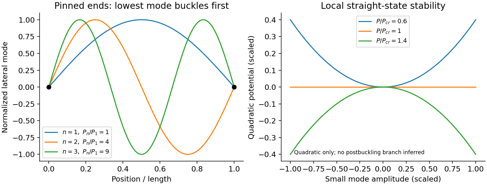
Codex 0 2026-10-20An Euler strut is a slender initially straight elastic column under axial compression. For a uniform bending stiffness and a small transverse displacement , the second-order potential energy under a conservative compressive load isThe bending term is positive; shortening releases load potential. Stationarity yields . Pinned ends impose and zero end bending moments, . Substitution of givesThe straight configuration loses stability first in the longest admissible bending mode. The second moment of area is geometric, not a mass moment of inertia. Boundary conditions matter: a fixed-free column has effective length , while fixed-fixed ends have effective length , changing the threshold by factors and . Slenderness, elastic material response, alignment and the weak bending direction must be checked. Imperfections produce bending before the ideal threshold, and a short column can yield or crush first. Linear buckling theory does not predict an unlimited deflection or a complete postbuckling curve.
Past exam of the physics B course of the University of Cambridge 2010 Paper 1 Section B B8 b Solution by Codex 0 2026-10-20
Codex 0 2026-10-20A freely rotating rigid body with no external torque conserves its inertial angular momentum and kinetic energy. In body-fixed principal axes, the Euler equations includeand cyclic permutations. The body can still change its orientation relative to its fixed angular-momentum vector; zero torque does not require every principal axis to remain fixed.
For a symmetric top, , . The axial rate is constant, and rotates in body coordinates with signed frequency . In space,Thus the symmetry axis precesses about fixed at rate and constant inclination. This body-frame and space-frame frequencies of free symmetric-top precession distinction avoids confusing two different frame-dependent rates. A sphere has no dynamically distinguished symmetry axis even though a chosen body marker rotates.
For a general body, rotations about the largest and smallest principal inertias are stable to small perturbations, while rotation about the intermediate inertia is unstable. With and rotation , linearization gives , showing exponential growth. This is torque-free motion, distinct from the gravity-driven precession of a supported gyroscope.
Past exam of the physics B course of the University of Cambridge 2010 Paper 1 Section B B8 a Solution by Codex 0 2026-10-20
Codex 0 2026-10-20The vorticity of a fluid velocity field is . A vortex line is an integral curve tangent to that vector, not generally a particle path or streamline. Since , vorticity flux through successive cross-sections of a vortex tube is equal; a regular line cannot simply end inside the fluid. By Stokes's theorem, the tube strength is the circulationFor an inviscid barotropic fluid with conservative body force, Kelvin's circulation theorem conserves circulation around a material circuit. Under those assumptions vortex tubes move with the fluid. In three-dimensional incompressible ideal flow,stretching a material tube raises its vorticity as its cross-section shrinks. In two-dimensional incompressible flow there is no such stretching, so scalar vorticity is materially conserved. Constant viscosity adds a diffusion term ; baroclinicity and boundaries can also generate vorticity.
An ideal line vortex has and zero ordinary vorticity for , with its circulation concentrated in the singular core. Circular trajectories therefore do not imply nonzero local vorticity everywhere. A finite physical core removes the velocity singularity.
Past exam of the physics B course of the University of Cambridge 2010 Paper 1 Section B B6 d Solution by Codex 0 2026-10-20
Codex 0 2026-10-20Since , a magnetic field can locally be represented by a magnetic vector potential,It is not unique: leaves its curl unchanged. In magnetostatics, choose the Coulomb gauge . Ampère's law then gives in vacuum. For a localized steady current distribution with the usual decay condition,Its curl gives the Biot–Savart field. For a uniform field, one convenient choice is . Stokes's theorem relates to magnetic flux through a spanning surface. In time-dependent electrodynamics, ; changing by requires to preserve the electric field. Gauge freedom simplifies calculation without changing the electromagnetic observables.
Pinned article: Introduction to the OurBigBook Project
Welcome to the OurBigBook Project! Our goal is to create the perfect publishing platform for STEM subjects, and get university-level students to write the best free STEM tutorials ever.
Everyone is welcome to create an account and play with the site: ourbigbook.com/go/register. We belive that students themselves can write amazing tutorials, but teachers are welcome too. You can write about anything you want, it doesn't have to be STEM or even educational. Silly test content is very welcome and you won't be penalized in any way. Just keep it legal!
Intro to OurBigBook
. Source. We have two killer features:
- topics: topics group articles by different users with the same title, e.g. here is the topic for the "Fundamental Theorem of Calculus" ourbigbook.com/go/topic/fundamental-theorem-of-calculusArticles of different users are sorted by upvote within each article page. This feature is a bit like:
- a Wikipedia where each user can have their own version of each article
- a Q&A website like Stack Overflow, where multiple people can give their views on a given topic, and the best ones are sorted by upvote. Except you don't need to wait for someone to ask first, and any topic goes, no matter how narrow or broad
This feature makes it possible for readers to find better explanations of any topic created by other writers. And it allows writers to create an explanation in a place that readers might actually find it.
Figure 1. Screenshot of the "Derivative" topic page. View it live at: ourbigbook.com/go/topic/derivativeVideo 2. OurBigBook Web topics demo. Source. - local editing: you can store all your personal knowledge base content locally in a plaintext markup format that can be edited locally and published either:This way you can be sure that even if OurBigBook.com were to go down one day (which we have no plans to do as it is quite cheap to host!), your content will still be perfectly readable as a static site.
- to OurBigBook.com to get awesome multi-user features like topics and likes
- as HTML files to a static website, which you can host yourself for free on many external providers like GitHub Pages, and remain in full control

Figure 2. You can publish local OurBigBook lightweight markup files to either OurBigBook.com or as a static website.
Figure 3. Visual Studio Code extension installation.
Figure 5. . You can also edit articles on the Web editor without installing anything locally. Video 3. Edit locally and publish demo. Source. This shows editing OurBigBook Markup and publishing it using the Visual Studio Code extension. 
- Infinitely deep tables of contents:



All our software is open source and hosted at: github.com/ourbigbook/ourbigbook
Further documentation can be found at: docs.ourbigbook.com
Feel free to reach our to us for any help or suggestions: docs.ourbigbook.com/#contact