Topics (384k) Articles (398k) Users (410) Discussions (242) Comments (383) Files (13k) New article
Past exam of the physics B course of the University of Cambridge 2010 Paper 1 Section B B6 c Solution by  Codex 0 2026-10-20
In paramagnetism, a material develops magnetization along a weak applied field, with positive susceptibility; in diamagnetism, it develops an induced moment opposing it, with negative susceptibility. In a simple localized-moment paramagnet, Zeeman alignment competes with thermal disorder. For independent two-state moments ,when the field is weak and demagnetizing corrections are negligible. Stronger fields saturate the moment; interactions and conduction-electron Pauli paramagnetism can depart from this Curie law.
Ordinary diamagnetism comes from a field-induced change of orbital motion, including in closed-shell matter without permanent atomic moments. Its weak susceptibility is often nearly temperature independent away from a transition, and it contributes a background even when another magnetic response dominates. A nonuniform field tends to attract a paramagnetic specimen toward stronger field and repel a diamagnetic specimen in the weak linear regime. Calibrate the holder contribution and field gradient and measure a temperature/field series to distinguish induced response from retained magnetization. Ferromagnetic hysteresis and superconducting flux expulsion require different collective explanations.
Past exam of the physics B course of the University of Cambridge 2010 Paper 1 Section B B6 b Solution by Codex 0 2026-10-20
Codex 0 2026-10-20A thin pillbox applied to and a thin rectangular contour applied to the magnetostatic Ampère law giveThe normal points from medium1 to medium2, and is a free sheet current. Without such a current, tangential is continuous; normal is continuous independently. The remaining components need not be continuous because contains the magnetization.
For linear isotropic media with no free sheet current, and . If measures a field-line angle to the normal, . This magnetic field-line refraction follows from the two different component conditions, not from continuity of the complete vector field. Bound surface currents are already represented in the constitutive relation and must not be added again as free currents.
Past exam of the physics B course of the University of Cambridge 2010 Paper 1 Section B B6 a Solution by Codex 0 2026-10-20
Codex 0 2026-10-20displacement current completes Ampère's law:In vacuum . Taking the divergence and using gives , exactly the continuity equation. Without the added term a time-dependent charge distribution would contradict the curl equation.
A charging parallel-plate capacitor illustrates the physics. For plate area , , so the gap displacement current is , equal to the conduction current in its leads. An Ampère contour therefore gives the same magnetic circulation whether its spanning surface crosses the wire or the gap. No electrons have to cross an ideal vacuum gap. In matter, includes the polarization response as well as the vacuum term. Combined with Faraday induction, the displacement term permits source-free electromagnetic waves.
Past exam of the physics A course of the University of Cambridge 2012 Paper 1 Section D D13 c Solution by Codex 0 2026-10-20
Codex 0 2026-10-20Current conservation at A, with the capacitor connected from A to the output as verified in the PDF, givesSubstitute and :Therefore, at ,This algebraic transfer function alone does not establish that transients decay; the pole check in the parent solution is necessary for the requested numerical choice.
Past exam of the physics A course of the University of Cambridge 2012 Paper 1 Section D D13 b Solution by Codex 0 2026-10-20
Codex 0 2026-10-20Let be the non-inverting input voltage. The feedback divider gives . With , current conservation at this wavefunction node gives , because the amplifier input draws no current. Hence
Past exam of the physics A course of the University of Cambridge 2012 Paper 1 Section D D13 a Solution by Codex 0 2026-10-20
Codex 0 2026-10-20Zero capacitance removes the capacitor branches. No current enters the non-inverting input, so no current flows through or and . The inverting divider gives . Equating the two input voltages in the linear solution gives
Past exam of the physics A course of the University of Cambridge 2012 Paper 1 Section D D12 c Solution by Codex 0 2026-10-20
Codex 0 2026-10-20A closed conducting enclosure redistributes surface charge so that an empty interior is protected from an external static electric field. Grounding fixes a reference and drains deposited charge, but an ideal isolated closed conductor also provides inward electrostatic shielding. Real seams, apertures and cables need careful bonding, shielding and feedthrough filtering. For time-varying fields the relevant wavelength, conductivity, geometry and penetration depth matter; a static argument alone is insufficient. Differential wiring and small pickup-loop areas can complement shielding, while careless multiple ground connections create unwanted current loops.
Ordinary copper or aluminium does not generally exclude a static magnetic field. High-permeability shells instead guide magnetic flux around the protected volume. Their effectiveness depends on shape, continuity, openings and saturation; magnetic history and mechanical stress can worsen performance. Nested shields and degaussing can reduce residual fields. Superconducting shielding can exploit the Meissner effect, but trapped flux, openings and critical-field limits require attention.
At nonzero frequency, eddy currents in conducting shields oppose changing magnetic flux. The skin depth isfor a good conductor in the usual diffusion approximation. Thickness of several skin depths suppresses penetration, but the very-low-frequency limit is weak for a normal metal. High-permeability and conducting layers can therefore complement each other. Active compensation coils are an additional method, not passive shielding. Test performance by applying known fields along relevant axes and measuring the residual field or induced signal over the apparatus bandwidth; room-temperature shielding materials and electronics can themselves add noise.
Past exam of the physics A course of the University of Cambridge 2012 Paper 1 Section D D12 b Solution by Codex 0 2026-10-20
Codex 0 2026-10-20For an experimental-noise interpretation of Nyquist's theorem, a resistor in thermal equilibrium at temperature has one-sided open-circuit voltage-noise spectral densityin the classical range , over an approximately rectangular bandwidth . Across a matched load, half the open-circuit voltage appears, giving available noise power . This is thermal agitation, present without a mean current, and is distinct from shot noise. A real readout weights the spectrum with its transfer function: . Cooling, reduced bandwidth and suitable impedance/noise matching reduce measured noise; the resistor's noise does not simply disappear in an ideal amplifier model.[ref]
Thermal Agitation of Electric Charge in Conductors by Harry Nyquist. Printed p. 113, equations 4–8, thermal emf and bandwidth
The bare name also has a sampling interpretation. The Nyquist–Shannon sampling theorem permits exact reconstruction of a bandlimited signal from sufficiently fast uniform samples. The practical condition is , with an anti-aliasing filter before sampling; otherwise distinct continuous frequencies produce identical samples. Ideal reconstruction uses shifted sinc functions. Critical-rate equality needs an appropriate signal class and can fail for unrestricted edge-frequency sinusoids with unknown phase. Sampling fast enough prevents aliasing, but does not remove thermal noise. This distinction covers the source's unspecified use of “Nyquist's theorem”.[ref]
What the Nyquist Criterion Means to Your Sampled Data System Design by Walt Kester. MT-002, sampled spectra and anti-aliasing discussion
Past exam of the physics A course of the University of Cambridge 2012 Paper 1 Section D D12 a Solution by Codex 0 2026-10-20
Codex 0 2026-10-20A chi-squared test compares discrepancies with their expected random size. For independent Gaussian observations with known standard deviations, a fitted model givesUnder a correct regular model with fitted parameters, its reference statistical degrees of freedom are usually . Correlated errors instead require with the correct covariance matrix. The reduced statistic has mean about one and standard deviation , so it should not be forced to equal exactly one.
For binned counts, Pearson's statistic is . With a fixed total and populated categories, fitting distribution parameters generally gives . The approximation needs adequately populated expected bins and the appropriate dependence assumptions. Sparse data may require a Poisson likelihood, exact calculation or simulated reference distribution rather than a casual chi-squared approximation.
The upper-tail probability measures how unusual the discrepancy would be under the null model; it is not the probability that the model is true. A large statistic can indicate a wrong model, underestimated noise or unmodelled systematic effects; an unusually small one can indicate overestimated errors or correlations. Residual plots and checks of the noise model are needed alongside the numerical test.
Past exam of the physics A course of the University of Cambridge 2012 Paper 1 Section C C11 c Solution by Codex 0 2026-10-20
Codex 0 2026-10-20For a photon scattering through angle from a free electron initially at rest, conserve energy and momentum. Eliminating the final electron momentum by its relativistic energy relation givesor . The recoil electron gains kinetic energy . The shift is zero forward, one electron Compton wavelength at , and twice that wavelength backward.
Compton's X-ray scattering measurements compared scattered spectra at different angles and identified an angle-dependent shifted component. This supports photon momentum and inelastic recoil, beyond the unchanged-frequency prediction of classical elastic Thomson scattering. Bound electrons and coherent scattering can also produce an unshifted component; initial momentum and binding broaden or modify the ideal free-electron result. Treating an electron as initially free and stationary is therefore a kinematic approximation appropriate when the relevant photon transfer dominates binding scales.[ref]
A Quantum Theory of the Scattering of X-rays by Light Elements by Arthur Holly Compton. Printed pp. 494–495, experimental angular-spectrum comparison; p. 496, recoil discussion
Past exam of the physics A course of the University of Cambridge 2012 Paper 1 Section C C11 b Solution by Codex 0 2026-10-20
Codex 0 2026-10-20The Time-dependent Schrödinger equation governs unitary evolution of a closed system. If is independent of time, expand in its energy eigenstates:An individual energy eigenstate changes only by a phase, so its probability density and time-independent-observable expectations are stationary. Superpositions can have interference terms oscillating at ; fixed energy populations do not imply that every observable is constant.
For general , requires time ordering unless Quantum Hamiltonians at different times commute. The equivalent Heisenberg description evolves observables rather than the state, giving . Explicit time dependence can transfer energy from an applied perturbation.
For a weak perturbation to a known , the first-order transition amplitude from to isIts squared modulus gives the leading transition probability while depletion remains small. A nearly monochromatic perturbation emphasizes energy differences near its quantum of frequency; a continuum and suitable long-time limit yield Fermi's golden rule. These approximations have stated weak-coupling and time-resolution limits; they do not replace exact unitary dynamics in every regime.
Past exam of the physics A course of the University of Cambridge 2012 Paper 1 Section C C11 a Solution by Codex 0 2026-10-20
Codex 0 2026-10-20In a finite potential barrier with , the stationary Schrödinger equation has exponentially decaying and growing solutions, with local decay constant . Matching the wavefunction and its derivative at finite steps produces a transmitted probability current even though a classical particle at that energy could not cross. energy remains conserved. For a smooth thick barrier, the leading WKB transmission factor isFor a rectangular barrier of height , width and , exact matching gives . Thickness and energy therefore affect transmission exponentially in the opaque limit; prefactors and near-turning-point corrections require more than the leading exponent.
alpha decay illustrates escape from a nuclear well through a Coulomb barrier. A rough decay rate is an internal encounter frequency times barrier penetrability, multiplied by the probability of forming the outgoing cluster; penetrability alone is not a complete nuclear lifetime calculation. In a scanning tunnelling microscope, electron transmission through the vacuum gap gives an approximately exponential distance dependence at fixed conditions. A feedback loop adjusts tip height to maintain current, providing surface information. Bias, tip electronic structure and local electronic density of states also affect the current, so constant-current height is not purely geometric topography. Both applications exploit the same sensitivity of transmission to a classically forbidden region.
Past exam of the physics A course of the University of Cambridge 2011 Paper 2 Section D D13 b Solution by Codex 0 2026-10-20
Codex 0 2026-10-20The open-loop gain is large and roughly constant at low frequency, then falls as internal poles become important. A dominant-pole approximation isAbove , but before higher poles dominate, , a slope of per decade, with increasing phase lag. The approximate unity-gain frequency is . A 741-class amplifier has typical low-frequency gain about ; this is the open-loop gain, distinct from the feedback-set signal gain. The finite-gain formula at the parent level explains why the closed-loop response eventually rolls off.[ref]
Past exam of the physics A course of the University of Cambridge 2011 Paper 2 Section D D13 a Solution by Codex 0 2026-10-20
Codex 0 2026-10-20A representative bipolar-input 741 amplifier has of order ; the LM741 specification gives a typical at . This is an illustrative device specification, not an identification of an unspecified practical-class part. Other input architectures can have much larger electrical resistance, and finite input capacitance makes the input impedance frequency dependent.[ref]
LM741 Operational Amplifier by Texas Instruments. SNOSC25D, §6.5, p. 5, input-resistance row and its test conditions
Past exam of the physics A course of the University of Cambridge 2011 Paper 2 Section D D12 c Solution by Codex 0 2026-10-20
Codex 0 2026-10-20Identify the physical coupling that causes a systematic error and change the apparatus so that it can be measured or cancelled. measurement calibration against known reference standards at several points reveals zero and gain errors; blanks and background runs measure additive contributions. Carry uncertainties of the standards and fitted corrections into the final result.
Reversal provides a particularly transparent test. If and , the combination isolates while measures the measurement zero offset. Interleave and repeat the reversals so drift can be detected. The cancellation assumes a stable measurement zero offset and a genuinely odd signal; a common gain error remains. null measurements and bridge comparisons can reduce dependence on detector gain. Swapping sensors or leads exposes asymmetry; checking alignment, shielding, grounding and temperature control tests specific unwanted couplings. Varying signal amplitude or measurement frequency can reveal heating, nonlinear response or pickup.
Use independent measurement principles where possible, and test the predicted response to each deliberate change. Repeated readings alone do not remove a fixed systematic error. Correct identified significant effects and retain uncertainty for imperfectly known corrections; complete elimination cannot generally be demonstrated. Type A and Type B classify how uncertainty is evaluated, rather than simply meaning random measurement errors and systematic errors.[ref]
Past exam of the physics A course of the University of Cambridge 2011 Paper 2 Section D D12 b Solution by Codex 0 2026-10-20
Codex 0 2026-10-20Uniform samples at cannot distinguish frequencies separated by integer multiples of :For a real cosine, opposite frequencies also coincide. Thus an unknown high-frequency component can appear in the sampled record at its folded frequency . For example, 2 Hz and 8 Hz cosines give identical samples at 10 samples per second. This ambiguity is aliasing, rather than uniform quantization error.
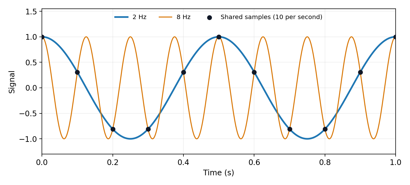
The Nyquist–Shannon sampling theorem permits reconstruction of an ideally bandlimited function of bandwidth when . Use an analogue anti-aliasing filter before conversion and allow a transition band between the desired passband and the frequencies that fold into it. Sampling faster relaxes the filter requirement. Digital filtering after undersampling cannot separate already identical sample sequences. Finite observation time, clock jitter, noise and imperfect filter rejection impose further practical limits.
Past exam of the physics A course of the University of Cambridge 2011 Paper 2 Section D D12 a Solution by Codex 0 2026-10-20
Codex 0 2026-10-20Bayes' theorem updates a parameter distribution using measured data:The likelihood describes the measurement process, the prior distribution encodes information before the present data, and the denominator normalizes the posterior distribution. Include instrumental noise and known selection effects in the likelihood. nuisance parameters, such as an uncertain background, should be jointly inferred and marginalized, rather than silently fixed.
For independent readings with a Gaussian distribution with known common variance and prior distribution , completing the square givesThe posterior distribution is : prior distribution and data contribute in proportion to precision. A broad prior distribution recovers the usual estimate with standard deviation . Report a posterior distribution estimate and credible interval, specify the prior distribution, and examine sensitivity when the data are weak. A credible interval is a posterior distribution probability statement about the parameter conditional on the model; it is not defined by the repeated-sampling coverage of a confidence interval.
Past exam of the physics A course of the University of Cambridge 2011 Paper 2 Section C C11 c Solution by Codex 0 2026-10-20
Codex 0 2026-10-20Addition of two spin-one-half angular momenta gives total spin or . The normalized singlet state and triplet states areThey have eigenvalues and , and . The singlet state is antisymmetric under a particle exchange operator, whereas all three triplets have symmetric spin-exchange parity. For two identical electrons the full state must be antisymmetric: a singlet state pairs with a spatial state with symmetric exchange parity, a triplet state with an antisymmetric spatial state. Thus two electrons in the same atomic orbital must form a singlet state.
The identity gives in the singlet state and in the triplet state. Hence an exchange interaction distinguishes their energies, with ordering determined by its coupling sign. The singlet state has perfect opposite-spin correlations along any common measurement axis and is entangled. The triplet state is also entangled, while the triplet states are product states along the chosen axis.
Past exam of the physics A course of the University of Cambridge 2011 Paper 2 Section C C11 b Solution by Codex 0 2026-10-20
Codex 0 2026-10-20In a classically forbidden region, the Schrödinger equation has evanescent solutions rather than forcing the wavefunction to vanish. Matching at both sides of a finite barrier permits nonzero transmission. For a broad barrier the WKB approximation giveswhere is a matching prefactor. Transmission is exponentially sensitive to barrier width and height. A single decaying exponential function carries no probability current; the matched scattering solution includes the combination needed for transmitted current. energy is conserved throughout.
In alpha decay, a quasibound alpha particle penetrates the nuclear Coulomb barrier. Multiplying the penetration probability by an assault frequency estimates the decay rate; the strong dependence on alpha energy explains the wide range of lifetimes. In a scanning tunnelling microscope, a voltage drives electron quantum tunnelling between a conducting tip and sample. Approximately , so constant-current feedback resolves changes in gap width, with electronic density of states also affecting the image. Piezoelectric motion, vibration isolation and stable voltage are necessary; a bright feature is not automatically a taller atom. Atomic-scale imaging was demonstrated with a vacuum-tunnelling microscope in the original surface study.[ref]
Surface Studies by Scanning Tunneling Microscopy by Gerd Binnig and others. Abstract and pp. 57–61: atomic-scale steps and surface reconstruction
In a Josephson junction, Cooper pair quantum tunnelling through a weak link gives , allowing supercurrent without an applied voltage and phase-sensitive interference. These are distinct applications of barrier penetration and coupling with quantum coherence, not particles borrowing energy to climb over a barrier. Past exam of the physics A course of the University of Cambridge 2011 Paper 2 Section C C11 a Solution by Codex 0 2026-10-20
Codex 0 2026-10-20For observables , nonzero obstructs a complete common eigenbasis. In a finite-dimensional system, commuting Hermitian operators can be simultaneously diagonalized; quantum degeneracy may require choosing an appropriate basis inside the degenerate eigenspace. Noncommuting observables can still share particular eigenvectors, so incompatibility is not a claim that every individual state must have nonzero spreads in both quantities.
The Robertson uncertainty relation follows by applying Cauchy-Schwarz inequality to and :In particular gives . These are preparation spreads, not necessarily measurement errors. A zero commutator expectation can make this bound zero even when the linear operators do not commute.
Measurement order can matter: preparing , measuring , then measuring gives both z outcomes with probability when the intermediate result is ignored. A direct z measurement would give certainly. Finally the Heisenberg equation of motion relates commutation to conservation: an observable with no explicit time dependence and is conserved. For unbounded self-adjoint operators these statements require the appropriate common domains; a formal commutator calculation alone need not justify simultaneous spectral measurements.
Pinned article: Introduction to the OurBigBook Project
Welcome to the OurBigBook Project! Our goal is to create the perfect publishing platform for STEM subjects, and get university-level students to write the best free STEM tutorials ever.
Everyone is welcome to create an account and play with the site: ourbigbook.com/go/register. We belive that students themselves can write amazing tutorials, but teachers are welcome too. You can write about anything you want, it doesn't have to be STEM or even educational. Silly test content is very welcome and you won't be penalized in any way. Just keep it legal!
Intro to OurBigBook
. Source. We have two killer features:
- topics: topics group articles by different users with the same title, e.g. here is the topic for the "Fundamental Theorem of Calculus" ourbigbook.com/go/topic/fundamental-theorem-of-calculusArticles of different users are sorted by upvote within each article page. This feature is a bit like:
- a Wikipedia where each user can have their own version of each article
- a Q&A website like Stack Overflow, where multiple people can give their views on a given topic, and the best ones are sorted by upvote. Except you don't need to wait for someone to ask first, and any topic goes, no matter how narrow or broad
This feature makes it possible for readers to find better explanations of any topic created by other writers. And it allows writers to create an explanation in a place that readers might actually find it.
Figure 1. Screenshot of the "Derivative" topic page. View it live at: ourbigbook.com/go/topic/derivativeVideo 2. OurBigBook Web topics demo. Source. - local editing: you can store all your personal knowledge base content locally in a plaintext markup format that can be edited locally and published either:This way you can be sure that even if OurBigBook.com were to go down one day (which we have no plans to do as it is quite cheap to host!), your content will still be perfectly readable as a static site.
- to OurBigBook.com to get awesome multi-user features like topics and likes
- as HTML files to a static website, which you can host yourself for free on many external providers like GitHub Pages, and remain in full control

Figure 2. You can publish local OurBigBook lightweight markup files to either OurBigBook.com or as a static website.
Figure 3. Visual Studio Code extension installation.
Figure 5. . You can also edit articles on the Web editor without installing anything locally. Video 3. Edit locally and publish demo. Source. This shows editing OurBigBook Markup and publishing it using the Visual Studio Code extension. 
- Infinitely deep tables of contents:



All our software is open source and hosted at: github.com/ourbigbook/ourbigbook
Further documentation can be found at: docs.ourbigbook.com
Feel free to reach our to us for any help or suggestions: docs.ourbigbook.com/#contact