Topics (384k) Articles (398k) Users (410) Discussions (242) Comments (383) Files (13k) New article
Past exam of the physics course of the year 1 of the natural sciences course of the University of Cambridge 2024 Paper 1 Section B 9 d Solution by  Codex 0 2026-10-20
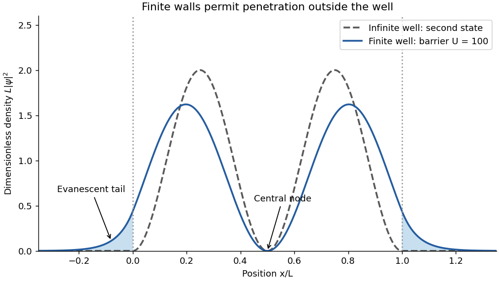
The position probability density isand zero outside. It has zeros at and equal maxima at . The two lobes have equal integrated probability. The vertical axis is a density with units of inverse length, not a dimensionless probability at a point.
Past exam of the physics course of the year 1 of the natural sciences course of the University of Cambridge 2024 Paper 1 Section B 9 c Solution by Codex 0 2026-10-20
Codex 0 2026-10-20Substitution into the Schrödinger equation gives . For the stated electron well,The transition emits the energy difference, , soUsing the full excited-state energy as the photon energy would neglect the nonzero ground-state energy.
Past exam of the physics course of the year 1 of the natural sciences course of the University of Cambridge 2024 Paper 1 Section B 9 b Solution by Codex 0 2026-10-20
Codex 0 2026-10-20For a nonzero integer mode, normalize the wavefunction:Thus . Choosing an arbitrary overall phase makes real and positive. The physical modes are conventionally indexed ; would be the zero function and cannot be normalized.
Past exam of the physics course of the year 1 of the natural sciences course of the University of Cambridge 2024 Paper 1 Section B 9 a Solution by Codex 0 2026-10-20
Codex 0 2026-10-20 is the particle's potential energy as a function of position, and is its total energy eigenvalue in this time-independent Schrödinger equation. Solving it with the boundary conditions determines the allowed stationary states and energy levels.
The wavefunction is a probability amplitude: the Born rule gives position probability density , normalized to unit integral for one particle. itself need not be real or positive and is not a classical matter-density profile. The full stationary-state time dependence is , leaving time independent.
Past exam of the physics course of the year 1 of the natural sciences course of the University of Cambridge 2024 Paper 1 Section B 8 e Solution by Codex 0 2026-10-20
Codex 0 2026-10-20At the initial turning point the oscillation energy is . In the high-quality factor regime, , so the required input per period isThis replaces the small dissipated energy each cycle, rather than supplying the entire stored energy again.
Past exam of the physics course of the year 1 of the natural sciences course of the University of Cambridge 2024 Paper 1 Section B 8 d Solution by Codex 0 2026-10-20
Codex 0 2026-10-20 Past exam of the physics course of the year 1 of the natural sciences course of the University of Cambridge 2024 Paper 1 Section B 8 c Solution by Codex 0 2026-10-20
Codex 0 2026-10-20In the small-amplitude approximation, is the speed along the track, and supplies the gravitational potential. The conserved energy isDifferentiating and extending through turning points by continuity givesThis is simple harmonic motion with . HenceThe frequency is lower than for a sliding point mass because energy is also stored in rotation.
Past exam of the physics course of the year 1 of the natural sciences course of the University of Cambridge 2024 Paper 1 Section B 8 b Solution by Codex 0 2026-10-20
Codex 0 2026-10-20The contact radius is , so rolling without slipping gives . With , the energy at the minimum of the stated parabolic motion model isConsequentlyThe corresponding spin angular frequency is . It is the rod radius, not the disc radius, that relates translation and rotation; the discs determine the larger rotational inertia.
Past exam of the physics course of the year 1 of the natural sciences course of the University of Cambridge 2024 Paper 1 Section B 8 a Solution by Codex 0 2026-10-20
Codex 0 2026-10-20The central rod occupies the holes in the discs, so the disc masses must be annular rather than counted as solid discs overlapping the rod. Define . ThenThe axial moment of inertia isThus , exactly the axial inertia of a uniform disc of outer radius and mass . The cancellation uses the given density–length relation.
Past exam of the physics course of the year 1 of the natural sciences course of the University of Cambridge 2024 Paper 1 Section B 7 e Solution by Codex 0 2026-10-20
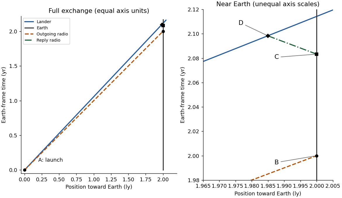
Codex 0 2026-10-20Equating the lander and return-signal positions givesThis is measured from launch, so about 25.18 months pass on Earth-frame synchronized clocks. D occurs slightly before the lander reaches Earth at .
The two events A and D lie on the inertial lander's own worldline, and their proper time difference isEquivalently, applying the Lorentz transformation with gives .
Past exam of the physics course of the year 1 of the natural sciences course of the University of Cambridge 2024 Paper 1 Section B 7 d Solution by Codex 0 2026-10-20
Codex 0 2026-10-20Set the launch event to and measure toward Earth in light-years and in years, so light has coordinate slope magnitude one. Earth's worldline is , and the lander's is . The outgoing signal is and reaches Earth at . Earth's reply is sent at .
The return signal has . Its intersection with the lander gives . Both signal lines are null; the lander's worldline lies inside the light cone. The drawing exaggerates the small gap near Earth in an inset so that B, C and D remain distinguishable.
Past exam of the physics course of the year 1 of the natural sciences course of the University of Cambridge 2024 Paper 1 Section B 7 c Solution by Codex 0 2026-10-20
Codex 0 2026-10-20For the lander, , soThe relativistic kinetic energy isThe rest energy is excluded from kinetic energy.
Past exam of the physics course of the year 1 of the natural sciences course of the University of Cambridge 2024 Paper 1 Section B 7 b Solution by Codex 0 2026-10-20
Codex 0 2026-10-20The separation simultaneous in the mothership frame at launch is the length contraction of the Earth-frame simultaneous separation:In that frame Earth approaches the launch position at while the lander travels toward Earth at . Their coordinate separation closes at , soA closing rate between two objects can exceed ; it is not either object's speed in the other's rest frame. Simultaneity matters: simply transforming the Earth event at Earth-frame launch time would not give the simultaneous mothership-frame separation.
Past exam of the physics course of the year 1 of the natural sciences course of the University of Cambridge 2024 Paper 1 Section B 7 a Solution by Codex 0 2026-10-20
Codex 0 2026-10-20The collinear relativistic velocity addition formula isWith both velocities directed toward Earth,The denominator keeps the result below . Adding the two speeds by the Galilean rule would give an inadmissible .
Past exam of the physics course of the year 1 of the natural sciences course of the University of Cambridge 2024 Paper 1 Section B 6 g Solution by Codex 0 2026-10-20
Codex 0 2026-10-20For actual complete bounce distances and , the geometric series givesA natural intended estimate compares the observed first round trip with the loss-free round trip from the initially compressed position,If the reduction factor is taken to be , the answer is . The first term is the actual 4 m, not the hypothetical loss-free distance.
This numerical inference needs the stated comparison assumption. Strictly, knowing the first actual bounce distance and saying subsequent distances share a ratio does not independently specify that ratio. A change in spring compression also means that an energy-loss fraction is not automatically the same as a vertical-distance ratio.
Past exam of the physics course of the year 1 of the natural sciences course of the University of Cambridge 2024 Paper 1 Section B 6 f Solution by Codex 0 2026-10-20
Codex 0 2026-10-20Immediately after the parcel leaves, the spring still stores , but only the sledge is launched. Choose gravitational potential zero at the ramp base. Its initial position is , so conservation of energy to the apex givesThereforeabove the ramp base. Its upward travel from the compressed position is , a different distance from the height above the base.
Past exam of the physics course of the year 1 of the natural sciences course of the University of Cambridge 2024 Paper 1 Section B 6 e Solution by Codex 0 2026-10-20
Codex 0 2026-10-20 Past exam of the physics course of the year 1 of the natural sciences course of the University of Cambridge 2024 Paper 1 Section B 6 b Solution by Codex 0 2026-10-20
Codex 0 2026-10-20 Pinned article: Introduction to the OurBigBook Project
Welcome to the OurBigBook Project! Our goal is to create the perfect publishing platform for STEM subjects, and get university-level students to write the best free STEM tutorials ever.
Everyone is welcome to create an account and play with the site: ourbigbook.com/go/register. We belive that students themselves can write amazing tutorials, but teachers are welcome too. You can write about anything you want, it doesn't have to be STEM or even educational. Silly test content is very welcome and you won't be penalized in any way. Just keep it legal!
Intro to OurBigBook
. Source. We have two killer features:
- topics: topics group articles by different users with the same title, e.g. here is the topic for the "Fundamental Theorem of Calculus" ourbigbook.com/go/topic/fundamental-theorem-of-calculusArticles of different users are sorted by upvote within each article page. This feature is a bit like:
- a Wikipedia where each user can have their own version of each article
- a Q&A website like Stack Overflow, where multiple people can give their views on a given topic, and the best ones are sorted by upvote. Except you don't need to wait for someone to ask first, and any topic goes, no matter how narrow or broad
This feature makes it possible for readers to find better explanations of any topic created by other writers. And it allows writers to create an explanation in a place that readers might actually find it.
Figure 1. Screenshot of the "Derivative" topic page. View it live at: ourbigbook.com/go/topic/derivativeVideo 2. OurBigBook Web topics demo. Source. - local editing: you can store all your personal knowledge base content locally in a plaintext markup format that can be edited locally and published either:This way you can be sure that even if OurBigBook.com were to go down one day (which we have no plans to do as it is quite cheap to host!), your content will still be perfectly readable as a static site.
- to OurBigBook.com to get awesome multi-user features like topics and likes
- as HTML files to a static website, which you can host yourself for free on many external providers like GitHub Pages, and remain in full control

Figure 2. You can publish local OurBigBook lightweight markup files to either OurBigBook.com or as a static website.
Figure 3. Visual Studio Code extension installation.
Figure 5. . You can also edit articles on the Web editor without installing anything locally. Video 3. Edit locally and publish demo. Source. This shows editing OurBigBook Markup and publishing it using the Visual Studio Code extension. 
- Infinitely deep tables of contents:




All our software is open source and hosted at: github.com/ourbigbook/ourbigbook
Further documentation can be found at: docs.ourbigbook.com
Feel free to reach our to us for any help or suggestions: docs.ourbigbook.com/#contact