Topics (384k) Articles (398k) Users (410) Discussions (242) Comments (383) Files (13k) New article
Past exam of the physics of the Earth as a Planet course of the University of Cambridge 2014 Paper 1 2 d Solution by  Codex 0 2026-10-20
Using the same diameter convention and viscosity estimate,Geometrical factors omitted in the scaling do not affect the conclusion: inertia is negligible. Convective inertia is smaller still by the small relief-to-wavelength ratio. Mantle creep is extremely slow despite the large length scale.
Past exam of the physics of the Earth as a Planet course of the University of Cambridge 2014 Paper 1 2 c Solution by Codex 0 2026-10-20
Codex 0 2026-10-20Assume the original ice sheet had time to reach local isostatic compensation, melted rapidly relative to subsequent rebound, and left one exponentially relaxing depression mode. Neglect elastic layering and assign the whole present gravity deficit to that unrelaxed depression. Load balance givesThe supplied sheet-gravity approximation gives the residual amplitudeFrom ,For an order-of-magnitude single-mode estimate, choose the ice-sheet diameter as wavelength, . Taking , the more accurate specified relation then givesA circular load has a spectrum, not one uniquely specified wavelength. Choosing instead gives about ; another wavelength convention rescales the answer linearly. The robust inference is viscosity of order within this simple model. A realistic estimate would also model gradual melting, other gravity anomalies, density interfaces, lithospheric flexure and depth-dependent mantle viscosity.
Past exam of the physics of the Earth as a Planet course of the University of Cambridge 2014 Paper 1 2 b Solution by Codex 0 2026-10-20
Codex 0 2026-10-20Unsteady inertial force density scales as , whereas viscous force density scales as . Using the preceding timescale givesConvective inertia has ratio . Since , this is smaller by for small relief. Thus the displayed estimate controls the larger inertial contribution in this model.
Past exam of the physics of the Earth as a Planet course of the University of Cambridge 2014 Paper 1 2 a Solution by Codex 0 2026-10-20
Codex 0 2026-10-20Subtract the background hydrostatic pressure. A relief amplitude produces a restoring pressure perturbation and horizontal gradient . Incompressibility makes the disturbance penetrate a depth of order its horizontal scale. For sinusoidal viscous rebound, with relaxation speed , the viscous force density is . Balancing givesThis is a small-amplitude viscous half-space estimate; numerical factors from the sinusoidal geometry are absent from a scaling argument.
Past exam of the physics of the Earth as a Planet course of the University of Cambridge 2014 Paper 1 1 g Solution by Codex 0 2026-10-20
Codex 0 2026-10-20A dense array does not correct an incorrect velocity model. The faster southwest block permits shorter travel times than an assumed uniform medium, with refraction favouring paths through fast rock. First arrivals may include refracted or seismic head wave paths rather than the assumed direct straight paths. Fitting those arrivals with one constant speed can make an earthquake on the fault appear closer to southwest stations and farther from northeast stations.
The sign follows even from a two-station linearization. Put southwest and northeast stations at , and the true event at with depth . In a constant-speed model,A negative observed differential residual therefore produces , an apparent southwest displacement. A common origin-time adjustment cannot remove this directional residual. The stated kilometre-scale offset is a model bias, not proof that the fault dips towards the apparent epicentres. Its exact magnitude cannot be predicted without the actual velocities and station geometry; the question supplies that magnitude as an observation.
The relevant contrast is independently documented at Parkfield: higher velocities lie southwest of the fault, with lower velocities northeast.[ref]
Scientific Advances at Parkfield by United States Geological Survey. Velocity-structure discussion, higher speeds southwest and lower speeds northeast
Account for the lateral structure and correct phases, then relocate and test whether the bias remains.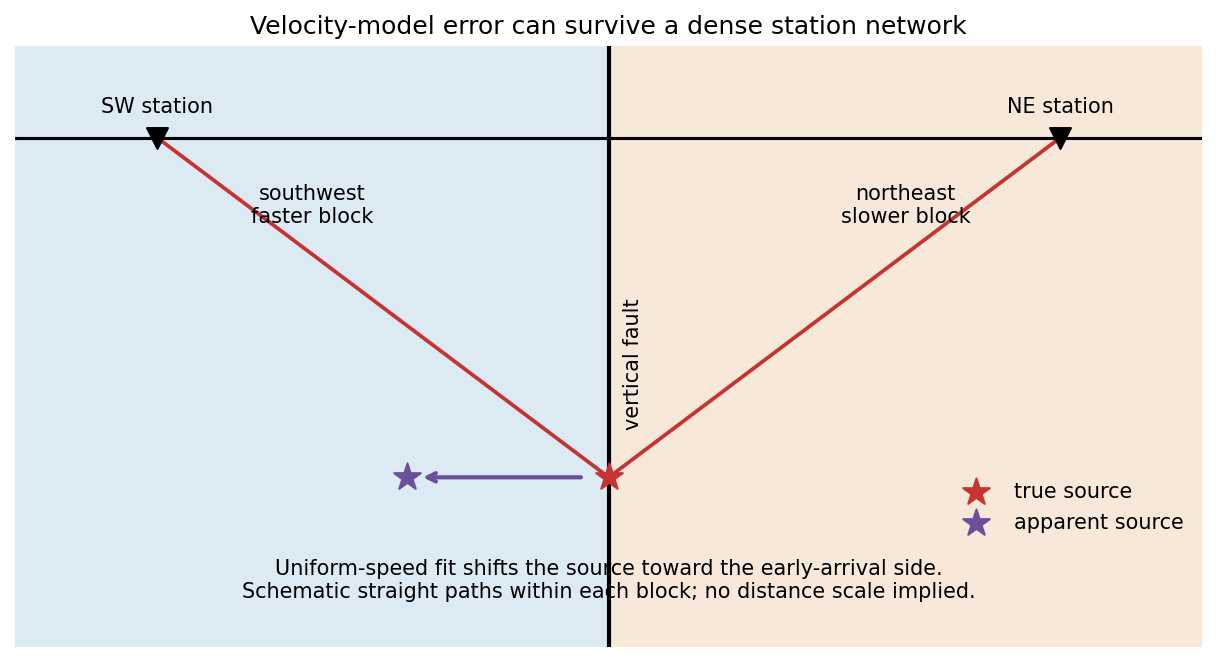
Past exam of the physics of the Earth as a Planet course of the University of Cambridge 2014 Paper 1 1 f Solution by Codex 0 2026-10-20
Codex 0 2026-10-20Let the seismic moment tensor of a double-couple seismic source be for perpendicular unit slip and normal vectors. Its T axis is , with eigenvalue , and its P axis is , with eigenvalue . They bisect the fault-plane and auxiliary-plane quadrants.
These earthquake pressure and tension axes describe the source deformation. They are not generally the principal axes of the ambient stress tensor. Friction, inherited fault orientation and local stress changes can rotate their relationship to that tensor; a stress inversion requires further assumptions and multiple mechanisms.
Past exam of the physics of the Earth as a Planet course of the University of Cambridge 2014 Paper 1 1 e Solution by Codex 0 2026-10-20
Codex 0 2026-10-20Nearby events observed at the same station share most of their propagation path, so common model and station errors cancel in differential arrival times. Waveform cross-correlation can also determine their relative timing more precisely than separate onset picks. Double-difference earthquake relocation fitsalong with the difference in origin times. The relative cluster geometry can be precise while the entire cluster remains displaced. Absolute anchoring still needs a well-calibrated velocity model or a source of known position.[ref]
A Double-difference Earthquake Location Algorithm: Method and Application to the Northern Hayward Fault, California by F. Waldhauser and W. Ellsworth. 2000, method and common-path rationale
Past exam of the physics of the Earth as a Planet course of the University of Cambridge 2014 Paper 1 1 d Solution by Codex 0 2026-10-20
Codex 0 2026-10-20Linearized arrivals contain . When the stations have similar depth sensitivities, a depth change shifts nearly all predicted times together and an origin-time change compensates it. Distant stations can also have very weak depth sensitivity. Improve the range of takeoff angles and station distances, especially with nearby or borehole stations, and include S–P or depth-phase differences such as pP–P that cancel origin time while retaining depth information. Accurate phase identification and the velocity model remain necessary.
Past exam of the physics of the Earth as a Planet course of the University of Cambridge 2014 Paper 1 1 c Solution by Codex 0 2026-10-20
Codex 0 2026-10-20For a double-couple seismic source, measure P-wave first-motion polarity signs and use source-to-station takeoff angles from the location and velocity model to plot them on a focal sphere. Fit the alternating radiation-sign quadrants, optionally adding amplitude ratios and waveform information. The two nodal planes determine a focal mechanism, conventionally expressed by fault strike, fault dip and fault rake.
A more general waveform inversion fits a seismic moment tensor to several components and stations. Its double-couple part supplies candidate slip and normal vectors, but a general moment tensor should not be forced to be double-couple without justification. Polarity calibration, near-nodal observations, path effects and takeoff-angle errors limit the result.
Point-source radiation alone interchanges the fault plane and auxiliary plane without changing the double couple. Resolve this fault-plane ambiguity using mapped rupture, aftershock geometry, geodesy or finite-rupture directivity. A dense set of polarity picks does not by itself remove that fundamental ambiguity.
Past exam of the physics of the Earth as a Planet course of the University of Cambridge 2014 Paper 1 1 b Solution by Codex 0 2026-10-20
Codex 0 2026-10-20Identify the event and pick calibrated P wave and, where available, S wave arrivals at stations of known position. Associate each pick with a seismic phase and uncertainty. An earthquake location by arrival times fitsfor the three hypocentre coordinates and earthquake origin time, using travel times from a specified velocity model. A grid search can initialize iterative weighted least squares or a probabilistic inversion. Station coverage must constrain depth as well as horizontal position; merely having four observations does not ensure a well-conditioned solution.
Errors include uncertain or misidentified onsets, clock and station-coordinate errors, wrong velocities or neglected three-dimensional structure, poor azimuthal coverage, inadequate station distances and depth–origin-time tradeoffs. Examine residual patterns and resolution, not only the minimum residual. A small formal covariance within a wrong velocity model can accompany a systematically biased hypocentre.
Past exam of the physics of the Earth as a Planet course of the University of Cambridge 2014 Paper 1 1 a Solution by Codex 0 2026-10-20
Codex 0 2026-10-20The hypocentre is the point where rupture begins. The epicentre is its projection onto the Earth's surface. An earthquake centroid is an effective spatial average of moment release over the rupture, with a corresponding mean release time. Initiation and average release need not occur at the same place or time, especially for an extended, asymmetric rupture.
Past exam of the physics of the Earth as a Planet course of the University of Cambridge 2013 Paper 1 3 d Solution by Codex 0 2026-10-20
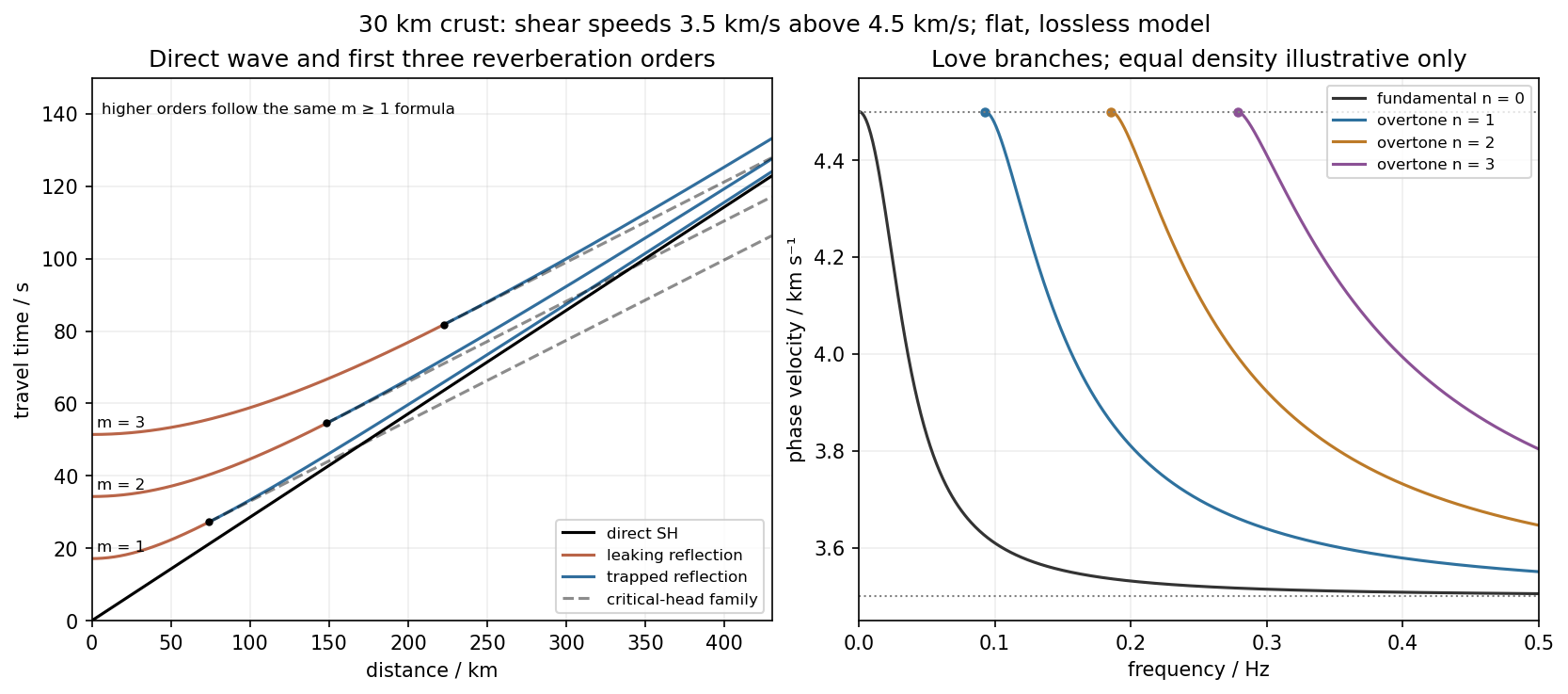
Codex 0 2026-10-20Use the flat two-layer model, with thickness , crustal shear speed and mantle speed . For SH-wave travel times in a crustal waveguide, unfolding each reflected path gives all reflection orders at once:with in kilometres and times in seconds. The direct wave begins at the origin; reflected orders have intercepts and approach the direct-wave slope at large distance.
The critical angle, measured from the vertical, is . Associated critical refraction and its multiples giveEach head-wave line is tangent to its reflection curve at the critical distance. In particular the primary head wave exists before it becomes the first arrival; it overtakes the direct wave only around .
The slope of a reflected travel-time curve is . For , , so the mantle supports outgoing shear radiation and successive reverberations leak energy. For , : the mantle field is evanescent and ideal interface reflection is total. These leaking and trapped SH-wave reverberations explain the annotations in the original travel-time drawing below. A reflected ray is not itself a separate Love mode: constructive interference of the trapped contributions, including reflection phase, selects the normal modes.
For a horizontally propagating mode with , define vertical wavenumbersThe free upper surface and welded interface impose the Love-wave dispersion conditionwhere are shear moduli. Each phase-velocity branch falls towards with increasing frequency. Higher branches join at their low-frequency cutoffs. At cutoff , soThus the first three overtones have maximum periods about , and . The fundamental mode has and no positive-frequency cutoff in this flat layer-over-half-space model: it approaches as , with ever-deeper penetration. The phase-velocity sketch uses an explicitly illustrative equal-density choice, because the question gives speeds but no density or rigidity ratio. That missing ratio changes detailed branch curvature, not the cutoff values or the requested branch topology.
For the actual finite spherical Earth, the very-long-period continuation must instead be described by discrete toroidal normal modes, not a flat infinite waveguide at arbitrary wavelength. The flat-model answer therefore does not assert a continuum of arbitrarily low-frequency global nonrigid oscillations. A global lowest oscillation frequency cannot be computed from the supplied crust-and-half-space data alone.[ref]
Essentials of Geophysics: Seismology by R. D. van der Hilst. §4.18, Love-wave trapping; §4.23, finite spherical Earth and discrete normal modes, especially printed pp. 184–187
Past exam of the physics of the Earth as a Planet course of the University of Cambridge 2013 Paper 1 3 c Solution by Codex 0 2026-10-20
Codex 0 2026-10-20The phase velocity in Figure 1 is measured along the Earth's surface. Spherical geometry makes the local horizontal phase speed at radius equal to . In the ray approximation, squared radial shear wavenumber isThe spherical surface-wave evanescence threshold immediately below the discontinuity is thereforeEquality is the grazing limit. Using directly would omit the requested spherical correction. Immediately above the discontinuity the corresponding boundary is . Hence the interval specifically describes propagation just above the jump and evanescence just below it. Slower modes can already be evanescent above .
Intersecting the plotted branches with gives the following approximate upper periods. Below each upper period, that branch is evanescent immediately beneath the discontinuity:
- fundamental mode: throughout the displayed – range;
- first and second overtones: approximately and ;
- successive higher curves: approximately , , , , and .
For these overtones the displayed ranges thus start near and end at their respective crossings. Any still higher curve already above the threshold at the lower plotted period has no evanescent interval within the displayed range. Readings of the closely spaced higher curves are only accurate to about a second, and the plot does not establish their continuation to unshown periods. Nor does the local inequality prove that a mode remains evanescent at every greater depth in an unspecified Earth model.
Past exam of the physics of the Earth as a Planet course of the University of Cambridge 2013 Paper 1 3 b Solution by Codex 0 2026-10-20
Codex 0 2026-10-20Write the oscillation period as , so locally . The first overtone is the lowest curve above the fundamental, not the fundamental mode itself. Near , Figure 1 gives approximately . Representative nearby readings are about at and at . ThusThe local group-velocity estimate isThese are graphical estimates, roughly and , rather than high-precision fitted constants. The nearby straight-line approximation need not describe that mode over the whole plotted period range. No source curve is reproduced here.
Past exam of the physics of the Earth as a Planet course of the University of Cambridge 2013 Paper 1 3 a Solution by Codex 0 2026-10-20
Codex 0 2026-10-20For group velocity from a period-dependent phase velocity, start with rather than equating group velocity to phase velocity. Differentiating,For the stated inverse-frequency term, , soThe inequality assumes positive frequency and physical positive phase velocity, with . The symbol here has units of acceleration and is unrelated to the plate thickness in Question 1.
Past exam of the physics of the Earth as a Planet course of the University of Cambridge 2013 Paper 1 2 b Solution by Codex 0 2026-10-20
Codex 0 2026-10-20Earthquake location. The hypocentre is rupture initiation; its surface projection is the epicentre. Record calibrated arrival times at stations of known coordinates, identify P wave and S wave phases, and predict their travel times through a stated velocity model. Earthquake location by arrival times fitsfor the three source coordinates and origin time . Linearization supplies residual equations . A grid search or iterative weighted least squares inversion can use pick uncertainties, while station geometry controls whether those parameters are well constrained. Four independent arrival constraints are the minimum for four unknowns, not a guarantee of a reliable solution.
In a homogeneous medium, an arrival-time difference between an S wave and a P wave cancels origin time and estimates source-to-station distance,Several distances intersect to locate the event; real layered or three-dimensional Earth structure requires curved-ray travel times. Nearby stations and diverse takeoff angles help resolve depth. Clock errors, phase misidentification, poor azimuthal coverage and incorrect velocities introduce uncertainty or systematic bias. Closely spaced earthquakes can be relocated precisely relative to each other because common-path errors partly cancel, even when their absolute locations remain uncertain. Report a location uncertainty and model assumptions, not merely a best-fit point.
H. F. Reid's earthquake-cycle model. A fault can remain locked while long-term tectonic motion slowly deforms the surrounding rocks. Elastic strain energy and shear stress accumulate. When resistance is overcome, rapid fault slip releases part of that stored energy as seismic waves, frictional heat and other irreversible work. The adjoining rocks partly recover their elastic distortion while retaining a permanent displacement discontinuity across the fault: this is elastic rebound. Surface markers initially crossing the fault become bent during loading and offset after slip.[ref]
Reid's Elastic Rebound Theory by United States Geological Survey. Explanation of gradual strain accumulation, sudden release and the displaced fence; cites Reid's 1910 report, especially pp. 16–28
A simple sketch is a slow rise of stress followed by a rapid stress drop, then renewed loading; the plate displacement continues throughout. Geodetic deformation, observed fault offsets and earthquake stress changes can test the picture. Actual cycles need not repeat with identical slips or times: creep, afterslip, stress transfer and heterogeneous friction complicate the idealization. The release need not remove all pre-existing stress. Elastic rebound explains storage and release; it is not a deterministic earthquake clock.
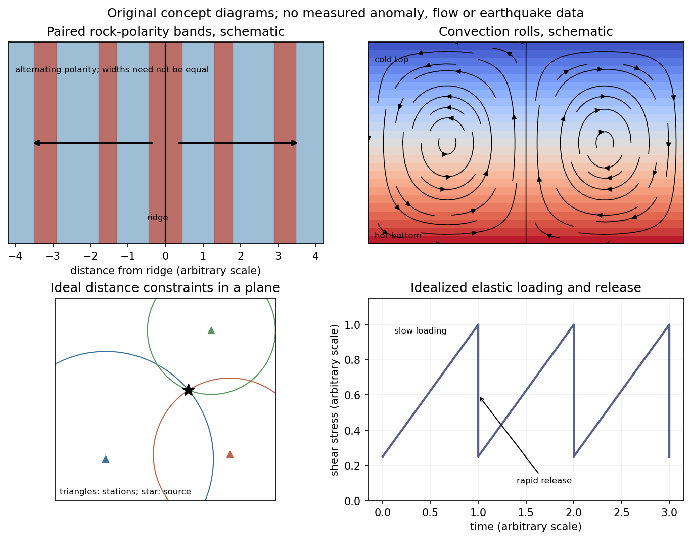
Schematic magnetic stripes, convection rolls, arrival-distance constraints and elastic loading–release cycle; no measured data
. Details. Past exam of the physics of the Earth as a Planet course of the University of Cambridge 2013 Paper 1 2 a Solution by Codex 0 2026-10-20
Codex 0 2026-10-20Oceanic magnetic anomalies. Newly formed oceanic crust contains magnetic minerals. As it cools through their magnetic blocking temperatures, it acquires thermoremanent magnetization recording the ambient field polarity. Continuing seafloor spreading carries that record away from the ridge. Geomagnetic reversals therefore generate approximately paired marine magnetic stripes parallel to the ridge, with older crust farther from its axis. A magnetometer measures the superposed field above this magnetized material; subtracting a reference field reveals magnetic anomalies. The anomaly sign and shape depend on magnetization direction, latitude, source depth and geometry, so a positive measured anomaly is not universally identical to normal rock polarity.[ref]
Developing the theory by United States Geological Survey. Sections Magnetic striping and polar reversals, and Seafloor spreading and recycling of oceanic crust
Matching a sequence of stripes to an independently dated reversal chronology gives plate ages and spreading histories. A stripe of width formed over interval implies half-spreading rate under steady symmetric spreading; full separation speed is . Unequal widths on opposite flanks can reflect asymmetric spreading or later deformation. Alteration, remagnetization and overlapping magnetic sources complicate inversion. The sequence correlation is stronger evidence than an isolated stripe or a field-strength peak.
Rayleigh-Bénard convection. Consider a horizontal fluid layer of thickness , hotter below by . The conductive state is motionless with a linear temperature gradient. A rising warm parcel is buoyant, but viscosity resists its motion and thermal diffusion erases its temperature anomaly. In the Boussinesq approximation, density variations are retained in buoyancy while the flow is otherwise incompressible. The competing effects are measured by the Rayleigh number and Prandtl number,For stress-free impermeable, fixed-temperature boundaries, linear stationary disturbances with horizontal wavenumber giveMinimizing gives and the critical Rayleigh number for an isothermal layer, . Two rigid no-slip, fixed-temperature boundaries instead give approximately ; the critical value is not independent of boundary conditions.[ref]
Boundary layer turbulence by Massachusetts Institute of Technology. Chapter 20, §20.4, critical value for two rigid isothermal plates
Above onset, buoyancy can sustain overturning rolls and heat transfer exceeds pure conduction, with Nusselt number . Nonlinear advection eventually limits the disturbance; larger driving can produce time-dependent or turbulent states. The ideal Boussinesq problem does not require hexagonal cells: planform selection depends on boundaries and non-Boussinesq effects. Convection driven by surface tension at a free surface is a distinct mechanism. An adverse temperature gradient supplies driving, but overcoming diffusion and viscosity requires a finite threshold.
Past exam of the physics of the Earth as a Planet course of the University of Cambridge 2013 Paper 1 1 e Solution by Codex 0 2026-10-20
Codex 0 2026-10-20The depth-averaged added horizontal compressive stress is . Resolving its traction on a plane dipping at angle gives the fault shear stress from a plate-integrated force,Keeping the previous topographic correction gives about . This is the mean additional shear from ridge push, assuming the force is transmitted through thickness and resolving the nonisotropic stress increment. An isotropic lithostatic pressure adds normal traction but no shear. The force integral alone does not specify the local stress at each point on the fault or establish failure.
Past exam of the physics of the Earth as a Planet course of the University of Cambridge 2013 Paper 1 1 d Solution by Codex 0 2026-10-20
Codex 0 2026-10-20Ridge push is a horizontal pressure force integrated with depth, equivalently a difference in gravitational potential energy per horizontal area. It is not the weight of a slab multiplied by the surface slope at one chosen point.
For an explicit compensated-column derivation, let measure depth below the ridge seafloor; the old seafloor is at . Set . The hot column has greater pressure. Its pressure excess over the old column isThe second line follows by integrating upwards from the compensation level. The two expressions agree at because . Integrating this positive pressure excess gives the ridge-push force in a plate model, directed away from the ridge:Consistently retaining only first order in thermal expansion givesIf the topographic term is retained within the same linear-density column model, it adds , giving . This is a useful small correction, not a claim that all other second-order material effects have been included. Both values use the intended hot initial plate, not the inconsistent printed zero-age profile.
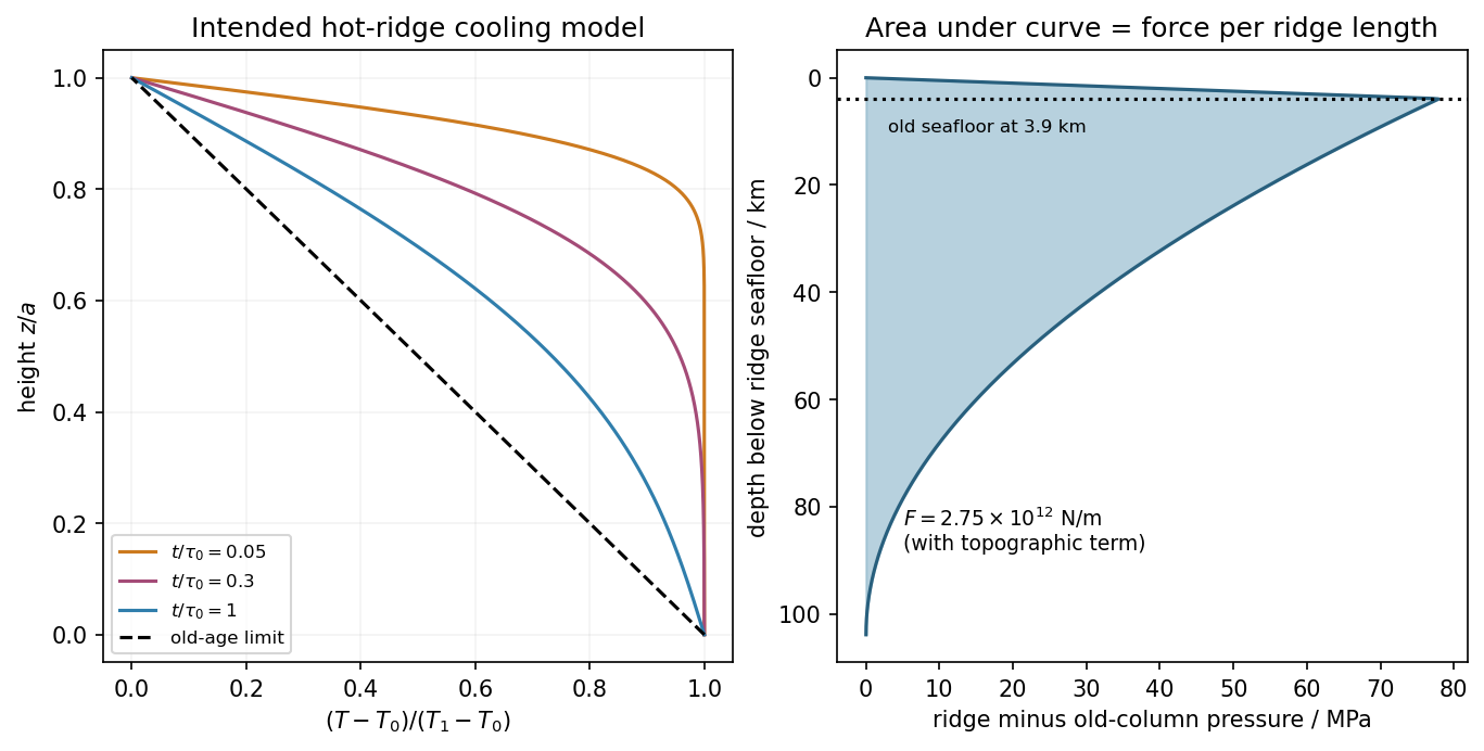
Hot-ridge and old-plate columns, and their compensated pressure difference in the intended cooling model
. Details. Past exam of the physics of the Earth as a Planet course of the University of Cambridge 2013 Paper 1 1 c Solution by Codex 0 2026-10-20
Codex 0 2026-10-20Use the intended hot-ridge state and a linear law of thermal expansion about mantle density at . Let be depth below the old seafloor. Its excess density isand its excess column mass is . Isostasy requires equal pressure at a compensation depth below both columns. Lowering the old seafloor by replaces rock by water, reducing column mass by . Therefore the isostatic ridge elevation in a plate model isHere ; the result is a first-order estimate and neglects sediments, crustal-composition differences and flexural support. If one instead insists on the literal printed zero-age profile, its column is denser than the old plate and the formal relative elevation reverses sign, to this order. That profile cannot describe the elevated hot ridge posited by the question.
Pinned article: Introduction to the OurBigBook Project
Welcome to the OurBigBook Project! Our goal is to create the perfect publishing platform for STEM subjects, and get university-level students to write the best free STEM tutorials ever.
Everyone is welcome to create an account and play with the site: ourbigbook.com/go/register. We belive that students themselves can write amazing tutorials, but teachers are welcome too. You can write about anything you want, it doesn't have to be STEM or even educational. Silly test content is very welcome and you won't be penalized in any way. Just keep it legal!
Intro to OurBigBook
. Source. We have two killer features:
- topics: topics group articles by different users with the same title, e.g. here is the topic for the "Fundamental Theorem of Calculus" ourbigbook.com/go/topic/fundamental-theorem-of-calculusArticles of different users are sorted by upvote within each article page. This feature is a bit like:
- a Wikipedia where each user can have their own version of each article
- a Q&A website like Stack Overflow, where multiple people can give their views on a given topic, and the best ones are sorted by upvote. Except you don't need to wait for someone to ask first, and any topic goes, no matter how narrow or broad
This feature makes it possible for readers to find better explanations of any topic created by other writers. And it allows writers to create an explanation in a place that readers might actually find it.
Figure 1. Screenshot of the "Derivative" topic page. View it live at: ourbigbook.com/go/topic/derivativeVideo 2. OurBigBook Web topics demo. Source. - local editing: you can store all your personal knowledge base content locally in a plaintext markup format that can be edited locally and published either:This way you can be sure that even if OurBigBook.com were to go down one day (which we have no plans to do as it is quite cheap to host!), your content will still be perfectly readable as a static site.
- to OurBigBook.com to get awesome multi-user features like topics and likes
- as HTML files to a static website, which you can host yourself for free on many external providers like GitHub Pages, and remain in full control

Figure 2. You can publish local OurBigBook lightweight markup files to either OurBigBook.com or as a static website.
Figure 3. Visual Studio Code extension installation.
Figure 5. . You can also edit articles on the Web editor without installing anything locally. Video 3. Edit locally and publish demo. Source. This shows editing OurBigBook Markup and publishing it using the Visual Studio Code extension. 
- Infinitely deep tables of contents:




All our software is open source and hosted at: github.com/ourbigbook/ourbigbook
Further documentation can be found at: docs.ourbigbook.com
Feel free to reach our to us for any help or suggestions: docs.ourbigbook.com/#contact