Topics (384k) Articles (398k) Users (410) Discussions (242) Comments (383) Files (13k) New article
Past exam of the physics course of the year 1 of the natural sciences course of the University of Cambridge 2015 Paper 1 Section B B9 b Solution by  Codex 0 2026-10-20
Boost along at into the centre-of-momentum frame. The composite is stationary. The incoming particle has , while the target has . After decay the two photons have energies and opposite momenta.
Equal laboratory photon energies require the rest-frame photons to have zero momentum component along the boost: must be equal for two opposite photons. Their directions are therefore and in the centre-of-momentum diagram, perpendicular to the incoming collision axis. Boosting those transverse photons gives exactly the laboratory momenta in part (a). A stationary composite has no direction-of-travel arrow in this frame.
Past exam of the physics course of the year 1 of the natural sciences course of the University of Cambridge 2015 Paper 1 Section B B9 a Solution by Codex 0 2026-10-20
Codex 0 2026-10-20In the laboratory frame the incoming particle and the composite move along , while the target is initially at rest. In the equal-energy two-photon decay of a moving particle, zero total transverse momentum makes the two photon directions symmetric about . Each photon has energy and momentum magnitude , so longitudinal momentum conservation gives . ThereforeTheir momenta can be written . The opening angle is not in this frame, because the parent carried nonzero total momentum.
Past exam of the physics course of the year 1 of the natural sciences course of the University of Cambridge 2013 Paper 1 Section E E15 c Solution by Codex 0 2026-10-20
Codex 0 2026-10-20In vacuum the electric and magnetic field energy densities areFor example, charging a capacitor requires . A parallel-plate capacitor with and then gives , identifying the electric field energy density. Similarly an inductor stores ; applying this to a long solenoid yields times its interior volume.
Electromagnetic energy is transported by the Poynting vector . Poynting's theorem,expresses local energy conservation and transfer to matter. In a vacuum plane wave , so the two energy densities are equal and the energy flux has magnitude . For nondispersive linear media the corresponding reversible expressions are and ; they must not be applied unchanged to arbitrary dispersive or hysteretic materials.
Past exam of the physics course of the year 1 of the natural sciences course of the University of Cambridge 2013 Paper 1 Section E E15 b Solution by Codex 0 2026-10-20
Codex 0 2026-10-20The Lorentz force determines the trajectory:Thus a magnetic field changes momentum direction but does no work; an electric field can change the particle's kinetic energy. In a uniform electric field with negligible magnetic field and nonrelativistic speed, is constant. A transverse initial velocity then gives a parabola.
In a uniform magnetic field, the parallel velocity is unchanged and the perpendicular motion is circular. Nonrelativistically,the combined trajectory is a helix, with circulation reversed when the charge sign reverses. Relativistically and the gyrofrequency is .
For perpendicular uniform fields in the magnetic-dominated case, the drift velocity is , which obeys . A particle at this velocity is undeflected: the crossed-field velocity selector selects speed in the appropriate direction, independent of mass and charge. Radiation reaction and collisions are neglected in these ideal trajectories.
Past exam of the physics course of the year 1 of the natural sciences course of the University of Cambridge 2013 Paper 1 Section E E15 a Solution by Codex 0 2026-10-20
Codex 0 2026-10-20A gravitational field is force per unit test mass, . Newton's law of universal gravitation gives the field of a point mass M:The potential is potential energy per unit mass, with zero at infinity for an isolated mass. Fields and potentials superpose. The potential difference fixes the work per unit mass, and a conservative gravitational field has zero circulation around a closed path.
For a continuous mass distribution, the gravitational Gauss law is . A spherical body therefore has the same exterior field as a point mass at its centre. Inside a uniform sphere of density ,The field is continuous at its surface and vanishes at its centre. An empty spherical shell has zero interior field but a nonzero constant interior potential. Near a small region of Earth's surface one may approximate as uniform and the potential change as . Farther away its spatial gradient produces tidal relative accelerations. Escape to infinity from radius R requires speed when rotation and other bodies are neglected.
Past exam of the physics course of the year 1 of the natural sciences course of the University of Cambridge 2013 Paper 1 Section D D12 c Solution by Codex 0 2026-10-20
Codex 0 2026-10-20Farther out, successive maxima and zeros occur at different angles for each wavelength. Many colour bands overlap, so the pattern becomes faint with increasingly washed-out colour contrast, rather than retaining a single sharp monochromatic fringe system. The overall single-slit intensity falls with an approximately inverse-square angular envelope.
Past exam of the physics course of the year 1 of the natural sciences course of the University of Cambridge 2013 Paper 1 Section D D12 b Solution by Codex 0 2026-10-20
Codex 0 2026-10-20The first zero of each colour is at . Blue therefore reaches its first zero closer to the axis than the reference green wavelength, and red reaches it farther away. At the reference colour is absent, while other wavelengths remain: there is no common black first minimum in white light. Adjacent regions change hue as different colour minima pass through them; wavelengths longer than the reference are still in their central maxima and tend to dominate near its first zero. The exact hue depends on the incident spectrum and spectral response.
Past exam of the physics course of the year 1 of the natural sciences course of the University of Cambridge 2013 Paper 1 Section D D12 a Solution by Codex 0 2026-10-20
Codex 0 2026-10-20At zero angle every slit element is in phase for every wavelength. Their central maxima coincide, so the centre is bright white. Shorter wavelengths have narrower central maxima; farther from the axis their contributions fade sooner, giving the central band reddish outer edges for a smooth white spectrum.
Past exam of the physics course of the year 1 of the natural sciences course of the University of Cambridge 2013 Paper 1 Section B B8 b Solution by Codex 0 2026-10-20
Codex 0 2026-10-20Between launch and interception, . The time-coordinate Lorentz transformation therefore givesThis is an elapsed coordinate time in B's inertial frame, not the travel time on A's clock. The latter would be .
Past exam of the physics course of the year 1 of the natural sciences course of the University of Cambridge 2013 Paper 1 Section B B8 a Solution by Codex 0 2026-10-20
Codex 0 2026-10-20 Past exam of the physics course of the year 1 of the natural sciences course of the University of Cambridge 2013 Paper 1 Section A 6 b Solution by Codex 0 2026-10-20
Codex 0 2026-10-20The laboratory mean lifetime is dilated to . Multiplying by the laboratory speed givesThis is the mean of the exponential decay-distance distribution, not a fixed distance travelled by every pion.
Past exam of the physics course of the year 1 of the natural sciences course of the University of Cambridge 2013 Paper 1 Section A 6 a Solution by Codex 0 2026-10-20
Codex 0 2026-10-20 Past exam of the physics course of the year 1 of the natural sciences course of the University of Cambridge 2013 Paper 1 Section A 1 b Solution by Codex 0 2026-10-20
Codex 0 2026-10-20The de Broglie wavelength fixes the same momentum , but the nonrelativistic electron has :Here , consistent with the stated nonrelativistic approximation. The photon energy and electron kinetic energy are not interchangeable.
Past exam of the physics course of the year 1 of the natural sciences course of the University of Cambridge 2013 Paper 1 Section A 1 a Solution by Codex 0 2026-10-20
Codex 0 2026-10-20 Past exam of the physics course of the year 1 of the natural sciences course of the University of Cambridge 2012 Paper 1 Section E E15 d Solution by Codex 0 2026-10-20
Codex 0 2026-10-20In vacuum, Maxwell's equations in SI units areThe displacement current term makes the last equation consistent with the charge continuity equation. In a source-free region, take the curl of Faraday's law and use . This givesA plane electromagnetic wave therefore propagates at . The divergence equations make both fields transverse; the curl equations giveThe electric fields and magnetic fields are in phase and perpendicular to one another and to the propagation direction. Their energy densities are equal:For electric-field peak amplitude , the time-averaged intensity is . Mutually coupled changing electric fields and magnetic fields transport energy through vacuum, even where no charges or conduction currents are present.
Past exam of the physics course of the year 1 of the natural sciences course of the University of Cambridge 2012 Paper 1 Section E E15 c Solution by Codex 0 2026-10-20
Codex 0 2026-10-20In electrostatic equilibrium a conductor has throughout its bulk and constant electric potential on each connected component. Otherwise free charge would continue moving. Gauss's law then excludes bulk excess charge; it resides on surfaces. Just outside a conductor the tangential field vanishes and the normal jump isfor a vacuum interface with outward normal . Surface charge rearranges in an external field to enforce these boundary conditions. Greater curvature often concentrates charge, but the actual distribution is a global boundary-value problem.
An empty closed cavity inside a conductor has constant potential and zero field, even in an external electrostatic field. If a charge is placed in the cavity, a Gaussian surface in the metal shows that the cavity wall carries total induced charge ; its detailed distribution depends on geometry. An initially neutral isolated conductor then has on its exterior surface. A grounded conductor can exchange charge with Earth, so this isolation condition no longer applies.
A useful example is a charge at height above an infinite grounded plane. In the physical half-space, the method of images replaces the induced charges by an image at height , giving the attractive force . The image is a mathematical construction, not an actual charge behind the conductor. Equipotential surfaces and charge conservation determine conductor fields together.
Past exam of the physics course of the year 1 of the natural sciences course of the University of Cambridge 2012 Paper 1 Section E E15 b Solution by Codex 0 2026-10-20
Codex 0 2026-10-20For two isolated point masses, introduce total mass , reduced mass and relative separation . The relative acceleration is . Conserved specific angular momentum fixes a plane and a constant areal velocity . The specific orbital energy isFor , the trajectory is a conic:Negative energy gives an ellipse, including the circular limit ; zero energy gives a parabola; positive energy gives a hyperbola. Bound ellipses obey andThus Kepler's laws of planetary motion follow from angular momentum conservation and the inverse-square force. For a circular orbit of radius , , while escape from that radius requires . Energy determines whether the orbit is bound; angular momentum also determines its shape. These ideal results neglect extended-body perturbations, drag and relativistic corrections.
Past exam of the physics course of the year 1 of the natural sciences course of the University of Cambridge 2012 Paper 1 Section E E15 a Solution by Codex 0 2026-10-20
Codex 0 2026-10-20An electric dipole consists of opposite charges separated by a small displacement, with electric dipole moment directed from negative to positive. At distances large compared with its size,The net charge term vanishes; the field decays faster than a monopole field. In an imposed slowly varying electric field,for a permanent fixed dipole. A uniform field produces a torque but no net force. For a linear induced dipole , the interaction energy is instead , because building the dipole also costs energy.
A small planar current loop has magnetic dipole moment , with the normal fixed by the right-hand rule. Outside the source,Magnetic field lines form closed loops; a current-loop dipole does not require magnetic monopoles. Dipole moments describe the leading directional field of a neutral localized source, and their torques explain alignment in external fields.
Past exam of the physics course of the year 1 of the natural sciences course of the University of Cambridge 2012 Paper 1 Section C C11 b Solution by Codex 0 2026-10-20
Codex 0 2026-10-20For free parallel RLC voltage decay, measure and branch currents from A to B. ThenThere is no external current, so Kirchhoff's current law gives . Differentiating yieldsFor the characteristic equation is . Its underdamped roots giveThe supplied inequality makes real. A real physical voltage has the general form , the real part of the printed complex expression. A general complex-valued solution uses both roots, . The inductor's initial current is fixed consistently by the undifferentiated current balance; it is not an arbitrary additional voltage-mode constant.
Past exam of the physics course of the year 1 of the natural sciences course of the University of Cambridge 2012 Paper 1 Section C C11 a Solution by Codex 0 2026-10-20
Codex 0 2026-10-20In sinusoidal steady state, complex impedance is the voltage phasor divided by the current phasor. Its modulus is the amplitude ratio and its argument is the voltage lead. With the convention, , so .
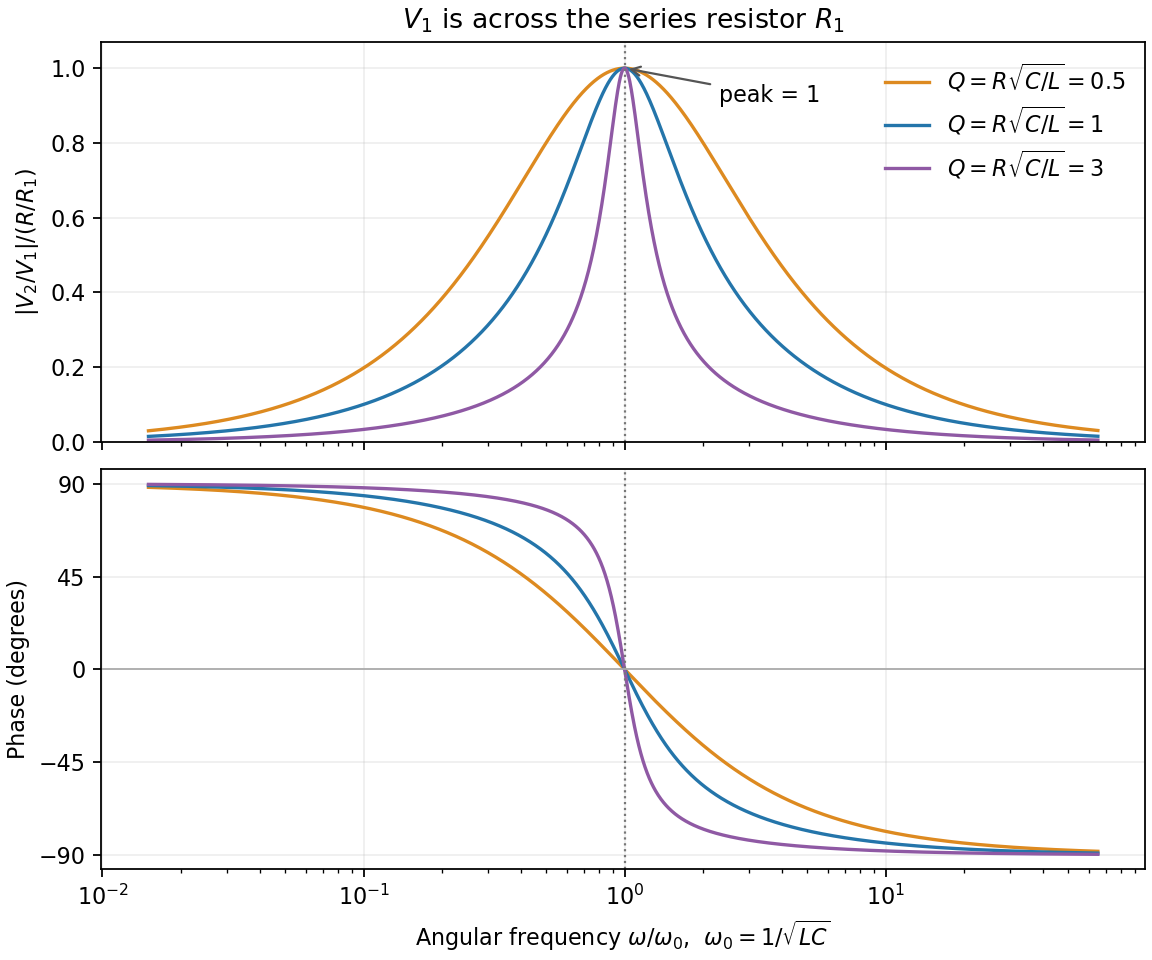
The PDF labels across , not across the complete driven network. If is the current through , then and , whereThe resistor-referenced parallel-resonator response isWriting ,The maximum occurs at , where and the phase is zero. Below resonance the phase is positive, tending to ; above it the phase is negative, tending to . The amplitude tends to zero at both extremes: the inductor shorts the parallel network at low frequency, and the capacitor does so at high frequency. At resonance their reactive currents cancel, leaving only the resistor current.
Pinned article: Introduction to the OurBigBook Project
Welcome to the OurBigBook Project! Our goal is to create the perfect publishing platform for STEM subjects, and get university-level students to write the best free STEM tutorials ever.
Everyone is welcome to create an account and play with the site: ourbigbook.com/go/register. We belive that students themselves can write amazing tutorials, but teachers are welcome too. You can write about anything you want, it doesn't have to be STEM or even educational. Silly test content is very welcome and you won't be penalized in any way. Just keep it legal!
Intro to OurBigBook
. Source. We have two killer features:
- topics: topics group articles by different users with the same title, e.g. here is the topic for the "Fundamental Theorem of Calculus" ourbigbook.com/go/topic/fundamental-theorem-of-calculusArticles of different users are sorted by upvote within each article page. This feature is a bit like:
- a Wikipedia where each user can have their own version of each article
- a Q&A website like Stack Overflow, where multiple people can give their views on a given topic, and the best ones are sorted by upvote. Except you don't need to wait for someone to ask first, and any topic goes, no matter how narrow or broad
This feature makes it possible for readers to find better explanations of any topic created by other writers. And it allows writers to create an explanation in a place that readers might actually find it.
Figure 1. Screenshot of the "Derivative" topic page. View it live at: ourbigbook.com/go/topic/derivativeVideo 2. OurBigBook Web topics demo. Source. - local editing: you can store all your personal knowledge base content locally in a plaintext markup format that can be edited locally and published either:This way you can be sure that even if OurBigBook.com were to go down one day (which we have no plans to do as it is quite cheap to host!), your content will still be perfectly readable as a static site.
- to OurBigBook.com to get awesome multi-user features like topics and likes
- as HTML files to a static website, which you can host yourself for free on many external providers like GitHub Pages, and remain in full control

Figure 2. You can publish local OurBigBook lightweight markup files to either OurBigBook.com or as a static website.
Figure 3. Visual Studio Code extension installation.
Figure 5. . You can also edit articles on the Web editor without installing anything locally. Video 3. Edit locally and publish demo. Source. This shows editing OurBigBook Markup and publishing it using the Visual Studio Code extension. 
- Infinitely deep tables of contents:



All our software is open source and hosted at: github.com/ourbigbook/ourbigbook
Further documentation can be found at: docs.ourbigbook.com
Feel free to reach our to us for any help or suggestions: docs.ourbigbook.com/#contact