Topics (384k) Articles (398k) Users (410) Discussions (242) Comments (383) Files (13k) New article
Past exam of the physics of the Earth as a Planet course of the University of Cambridge 2016 Paper 1 3 a Solution by  Codex 0 2026-10-20
For uniform density and stiffness, linear momentum balance without body force is . The minor elastic symmetries make the two symmetric-strain terms equal, so . Write and . Then and . Thus a nontrivial plane-wave profile satisfiesThe density-normalized elastic acoustic tensor is consequentlyThe alternative dummy-index form is identical. In ordinary conservative elasticity, major symmetry gives after interchanging the dummy indices. This symmetry comes from a strain-energy density; it is an assumption of the ordinary elastic tensor, not a consequence of homogeneity alone.
For any such eigenpair the profile is arbitrary, since both sides carry the same . This nondispersive result uses linear, local, time-independent elasticity without attenuation or spatial dispersion. A profile with is a trivial uniform or affine displacement field and cannot be used by itself to infer the wave-speed eigenvalue condition.
Past exam of the physics of the Earth as a Planet course of the University of Cambridge 2016 Paper 1 2 b Solution by Codex 0 2026-10-20
Codex 0 2026-10-20First-motion source mechanisms. Locate an earthquake from arrival times and use a seismic velocity model to calculate each station's source takeoff direction. Measure the initial direct P wave polarity after checking instrument sign, component orientation, timing and phase identification. An upward trace at an instrument is not automatically a source compression without the propagation and component convention. Plot the inferred source radiation signs on a focal sphere, commonly using a lower-hemisphere equal-area projection, and seek nodal planes separating positive and negative observations.
For a shear dislocation with orthogonal unit slip and fault-normal vectors , the double-couple fault source has . Its far-field P radiation sign is that ofThe two zeros are orthogonal nodal planes; the four quadrants alternate between outward and inward initial radiation. Their orientations and quadrant signs determine candidate strike, dip and rake. Normal, reverse and strike-slip mechanisms give different projected patterns. The earthquake pressure and tension axes are the negative and positive moment-tensor principal directions, respectively; they do not by themselves measure the complete regional stress tensor.
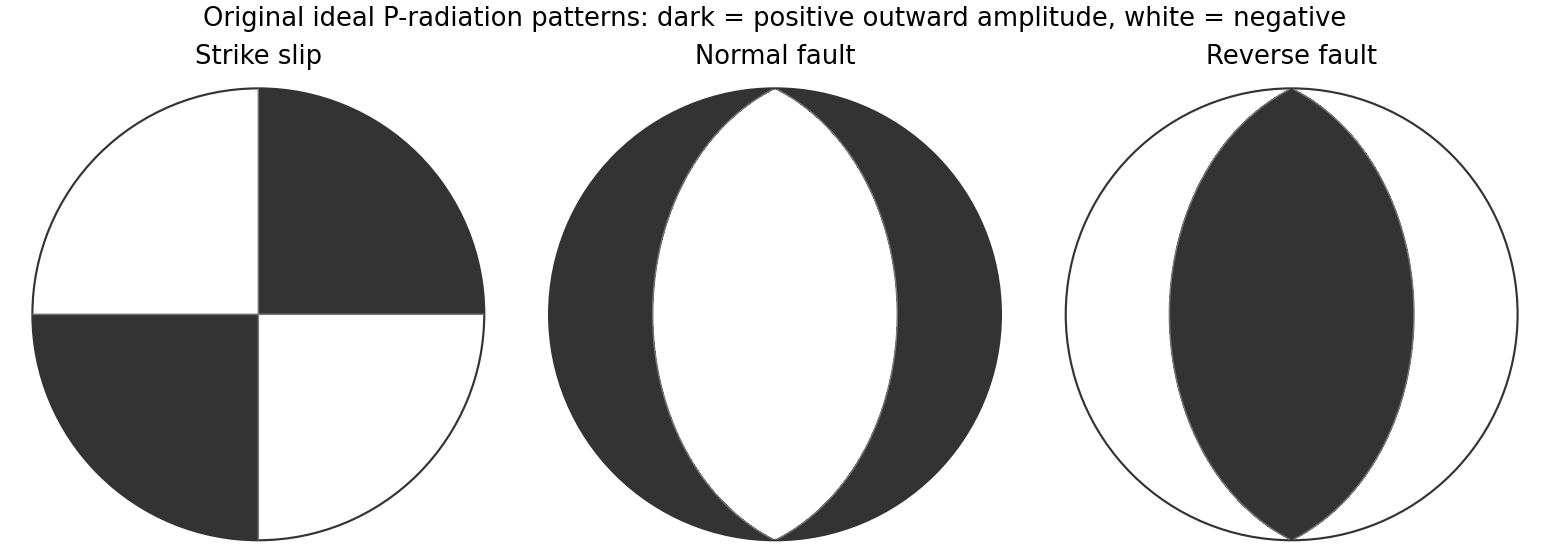
Original lower-hemisphere equal-area P-radiation polarity examples for ideal strike-slip, normal and reverse double couples
. Details. There is a fundamental fault-plane ambiguity: exchanging and leaves the radiation tensor unchanged. First motions therefore give a fault plane and an auxiliary plane without saying which actually slipped. Use mapped rupture, aftershock geometry or independent geodetic displacement to select the physical fault where possible. Polarity signs alone do not measure scalar seismic moment, source duration or rupture extent. A poorly sampled focal sphere or many near-nodal observations can admit several mechanisms rather than one defensible beachball.
Propagate uncertainty in event depth, velocity gradients and takeoff angles, allow for mispicked or reversed polarities, and report the range of mechanisms consistent with the observations. A primary method did this by testing alternative locations and velocity models and validated its uncertainty estimates using noisy synthetic data and clusters of events with similar waveforms.[ref]
A New Method for Determining First-Motion Focal Mechanisms by Jeanne L. Hardebeck and Peter M. Shearer. pp. 2264–2266 and abstract, first-motion construction, polarity/takeoff uncertainty and independent validation tests
Broadband waveforms and amplitude ratios add information, especially for non-double-couple sources, but they are additional measurements rather than a way to extract amplitude information from a sign-only data set.Radial density structure. In an isotropic adiabatic material, the seismic parameter isFor a chemically homogeneous region whose background stratification is adiabatic, . Combine this with spherical hydrostatic balance and mass conservation to obtain the Adams-Williamson equationsThe inward density increase follows compressibility under the increasing pressure. A specified starting density and measured allow integration within a homogeneous adiabatic layer. Seismic velocities alone, however, do not determine that density normalization, since they contain ratios of moduli to density. Chemical boundaries, phase transitions, nonadiabatic thermal gradients and anisotropy require additional modeling; a composition jump is not obtained by blindly integrating the smooth relation across it.
Use travel times and surface waves to constrain elastic velocities, reflected/converted phases to locate interfaces, and normal-mode frequencies to constrain density as well as elastic structure through their sensitivity kernels. Impose independently known total mass and moment of inertia:Because these weight depth differently, they help distinguish admissible profiles, but two integrals alone do not specify an arbitrary radial function. Laboratory equations of state and mineral physics restrict composition, compressibility and density jumps. pressure and enclosed mass are matched across interfaces, while density may jump. In a liquid region and , so the shear-wave absence constrains phase state without itself providing a direct density measurement.
The Preliminary Reference Earth Model is a concrete joint inversion of seismic travel times, normal modes, mass and inertia, including density and attenuation along with elastic structure. The original analysis combined these complementary data rather than deriving density uniquely from P wave speed.[ref]
Preliminary reference Earth model by Adam M. Dziewonski and Don L. Anderson. abstract and pp. 297–300, data classes and coupled radial reference-model inversion
A defensible radial density model combines hydrostatic/thermodynamic relations with seismic and global integral constraints, and states where homogeneity and adiabaticity fail. Past exam of the physics of the Earth as a Planet course of the University of Cambridge 2016 Paper 1 2 a Solution by Codex 0 2026-10-20
Codex 0 2026-10-20gravity and surface topography. gravity responds to all density structure, while surface topography records both load and support. First specify the reference field and measurement height. latitude and planetary rotation affect normal gravity. At elevation , the reference field decreases approximately by ; a free-air gravity anomaly restores this elevation effect but retains topographic mass. A Bouguer gravity anomaly additionally subtracts an approximate topographic slab contribution . terrain correction replaces the unrealistic slab near valleys and ridges, and spherical geometry matters over large areas. A density choice is required for these reductions; a numerical crustal density is not provided here.
In Airy isostasy, surface topography of height and crustal density is compensated by a root of thickness replacing mantle of density . Equal column masses give . The positive gravity of the relief is partly cancelled by the negative density contrast of the root. At long wavelengths a compensated mountain can therefore have a modest free-air anomaly and a negative Bouguer anomaly. Pratt isostasy instead varies column density at a roughly common compensation depth. Neither model says that surface topography itself exerts no gravity.
Potential-field depth filtering makes wavelength crucial. In a planar Fourier approximation, a density interface at depth is attenuated by at horizontal wavenumber . For a small Airy-compensated height perturbation and a compensation interface at depth , the gravity-topography admittance is approximatelyLong wavelengths allow strong cancellation between load and root. At short wavelengths the root's gravity is filtered out, so the observed near-surface mass can dominate even if the column is compensated. In a flexural isostasy model, an elastic lithosphere supports and spreads the load; for downward deflection and imposed load , , with . Thus , and the effective elastic thickness controls the support scale.
Estimate admittance from cross-spectra of gravity and surface topography, and compare its wavelength dependence and coherence with local-compensation, elastic-flexure and subsurface-load models. A primary Atlantic study sampled ship-track free-air gravity and bathymetry and compared their Fourier-domain relationship with compensation models, illustrating this observational route rather than inferring a root from the sign of one gravity value.[ref]
The relationship between bathymetry and gravity in the Atlantic Ocean by Dan McKenzie and Carl Bowin. pp. 1903–1915, ship-track sampling, spectral transfer estimates and wavelength-dependent compensation
Check navigation, instrument drift, terrain/density reductions, sediment and water loads, and independent seismic crustal constraints. Density-depth trade-offs and mantle dynamic support make the inverse problem nonunique; surface topography and gravity together constrain support, but do not uniquely map every density anomaly.mantle viscosity. A second, independent route concerns deformation rates rather than static compensation. glacial isostatic adjustment follows loading and unloading of a deformable Earth: an ice sheet depresses the surface, and subsequent removal leaves time-dependent uplift, horizontal displacement, sea-level and gravity changes. Fit dated relative sea-level indicators and raised shorelines together with geodetic displacement rates and a reconstructed ice/water load history to a viscoelastic Earth model. Relative sea level includes solid-surface motion, changing geoid and redistribution of ocean water; treating it only as local vertical rock motion biases the inference.
For scale, a sinusoidal surface perturbation of wavenumber on a uniform incompressible viscous half-space relaxes under gravity with . A Maxwell material separately has a stress-relaxation scale . These are different experiments and generally different times: rebound modes also involve gravity, spherical geometry, a layered mantle and elastic lithosphere. Fit a family of relaxation modes or a full load-history convolution, rather than equating every observed rebound time to .
Use independent ice-margin, exposure-age and sea-level constraints to reduce the trade-off between ice history and viscosity; compare horizontal as well as vertical GNSS motions, and separate present ice loss, groundwater changes and tectonic signals from the older loading response. A primary global analysis jointly tested ice-history and mantle-response predictions against space-geodetic observations, rather than treating a local uplift rate as a unique viscosity measurement.[ref]
postseismic relaxation probes shallower or faster relaxation after a stress perturbation, but must be distinguished from afterslip and poroelastic deformation. Long-wavelength geoid and mantle-flow models provide complementary constraints when density structure is estimated independently from seismic structure and mineral physics; unknown density-to-velocity conversion and boundary tractions remain trade-offs. Laboratory creep experiments constrain constitutive laws as functions of temperature, stress and grain size, but require a large extrapolation to geological conditions. Combine spatially and temporally distinct observations; there is no single directly measured mantle viscosity independent of depth, rheology and loading assumptions.
Past exam of the physics of the Earth as a Planet course of the University of Cambridge 2016 Paper 1 1 e Solution by Codex 0 2026-10-20
Codex 0 2026-10-20Assume an Earth-like reversing planetary magnetic field and magnetizable crust that acquires thermoremanent magnetization on cooling. Alternating polarity intervals then produce marine magnetic stripes parallel to each spreading ridge, with matching age/polarity sequences on its two sides. AB has half-spreading rate 10 mm/year, whereas AC has half-spreading rate 24 mm/year. Thus the same polarity interval produces widths and mm when time is in years: the AC stripes are 2.4 times wider. Age increases away from each ridge. The transform produces no new crust; bands end or are displaced at it, rather than forming a third symmetric stripe sequence centred on BC. This is the remanent-magnetization/spreading mechanism developed from marine magnetic observations.[ref]
Magnetic Anomalies Over Oceanic Ridges by F. J. Vine and D. H. Matthews. pp. 947–949, alternating remanent magnetization and the spreading interpretation
A more precise local sketch can be made in the northern junction frame. Let be distances in kilometres along the fixed tangent axes and the crustal age in Myr; numerically, mm/year equals km/Myr. Relative to the moving junction, the velocities are , and . In A the steady age field is , since backwards advection first reaches either the AC or AB ridge. Equal-age bands therefore join as right-angle corners within A, with the corners migrating along the ray . In the B wedge, and the stripes meet the transform. On the C flank directly supplied from AC, ; other parts of C carry older crust whose inherited pattern requires earlier boundary history.
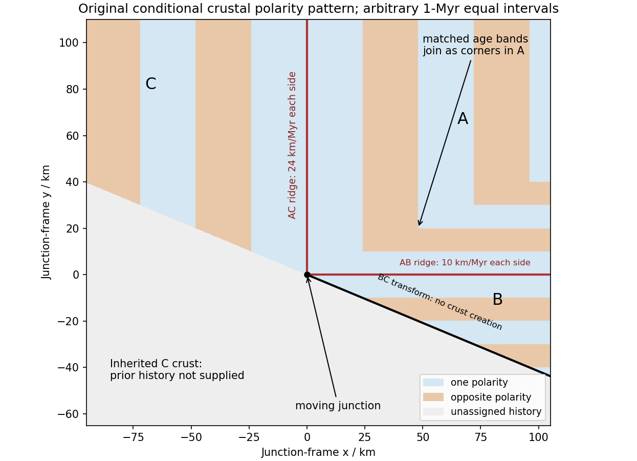
Original conditional remanent-polarity sketch in the north-junction frame; reversal intervals are illustrative and unsupplied older crust is left unassigned
. Details. The sketch displays magnetization polarity, not a computed total-field anomaly amplitude. Actual anomalies depend on the planetary field direction, source depth, magnetization strength and observation geometry. The paper supplies no field history, so a numerical reversal chronology or an absolute positive/negative anomaly sequence cannot be inferred. Without field reversals, ridge accretion alone does not imply alternating polarity stripes.
Past exam of the physics of the Earth as a Planet course of the University of Cambridge 2016 Paper 1 1 d Solution by Codex 0 2026-10-20
Codex 0 2026-10-20At the north pole , so the velocities reverse:The triangle still has side lengths 20, 48 and 52 mm/year. Across AB, A moves toward positive relative to B; across AC, A moves toward positive relative to C. Both boundaries therefore open and are spreading ridges, with full opening speeds 20 and 48 mm/year. Together with BC they form a ridge-ridge-transform triple junction.
In the symmetric normal-spreading model, a ridge's normal velocity is the mean normal velocity of its two plates. AB gives , and AC gives . Their intersection lies on the BC transform velocity line:This northern junction is also instantaneously kinematically stable. The diagrams use the same fixed geocentric tangent axes at both poles; reversing velocities is not the same operation as reflecting a map drawn from an exterior observer's viewpoint.
Not every ridge-ridge-transform geometry works. For pure normal spreading, each ridge velocity line is the perpendicular bisector of the corresponding side of the plate velocity triangle. Their intersection is the triangle's circumcenter. A transform junction must also lie on the third side's line. A nondegenerate triangle's circumcenter lies there only at that side's midpoint, so the opposite angle is a right angle. Equivalently, . The two ridge directions are then perpendicular, as they are here. RRF junctions are conditionally stable, with the right-angle ridge geometry in this symmetric pure-normal model; they are not all stable. Oblique or asymmetric accretion changes the velocity-line assumptions and must be specified separately.
Past exam of the physics of the Earth as a Planet course of the University of Cambridge 2016 Paper 1 1 c Solution by Codex 0 2026-10-20
Codex 0 2026-10-20At the south pole . Choose plate C as the instantaneous reference frame. Since mm, the two components of relative angular speed give 20 and 48 mm/year. The plate velocities in the fixed tangent-plane axes areThe plate velocity triangle therefore has sidesThe physical boundary rays point along for AB, for AC and for BC. Plate A occupies the quadrant between the first two rays, B the narrow wedge between AB and BC, and C the remainder. The stated overriding relations make AB and AC subduction trenches, while BC remains a transform fault: this is a trench-trench-transform triple junction. Put the subduction teeth on B's side of AB and A's side of AC, identifying B above A and A above C.
For kinematic stability there must be a single junction velocity compatible with all three boundary-normal motions. Use the standard idealization that each trench's normal velocity is that of its overriding plate, with no independent rollback. AB is parallel to , so . AC is parallel to , so . The transform requires to be parallel to , which is true for this intersection. HenceThe southern triple junction is instantaneously kinematically stable. It is stationary relative to B, migrates along AB relative to A, and migrates along BC relative to C. This compatibility result does not promise long-term stability if plate rotations or trench rollback change. Notice that the three relative velocities close even though the overriding order is not a statement that all three plates move toward one common stationary point.
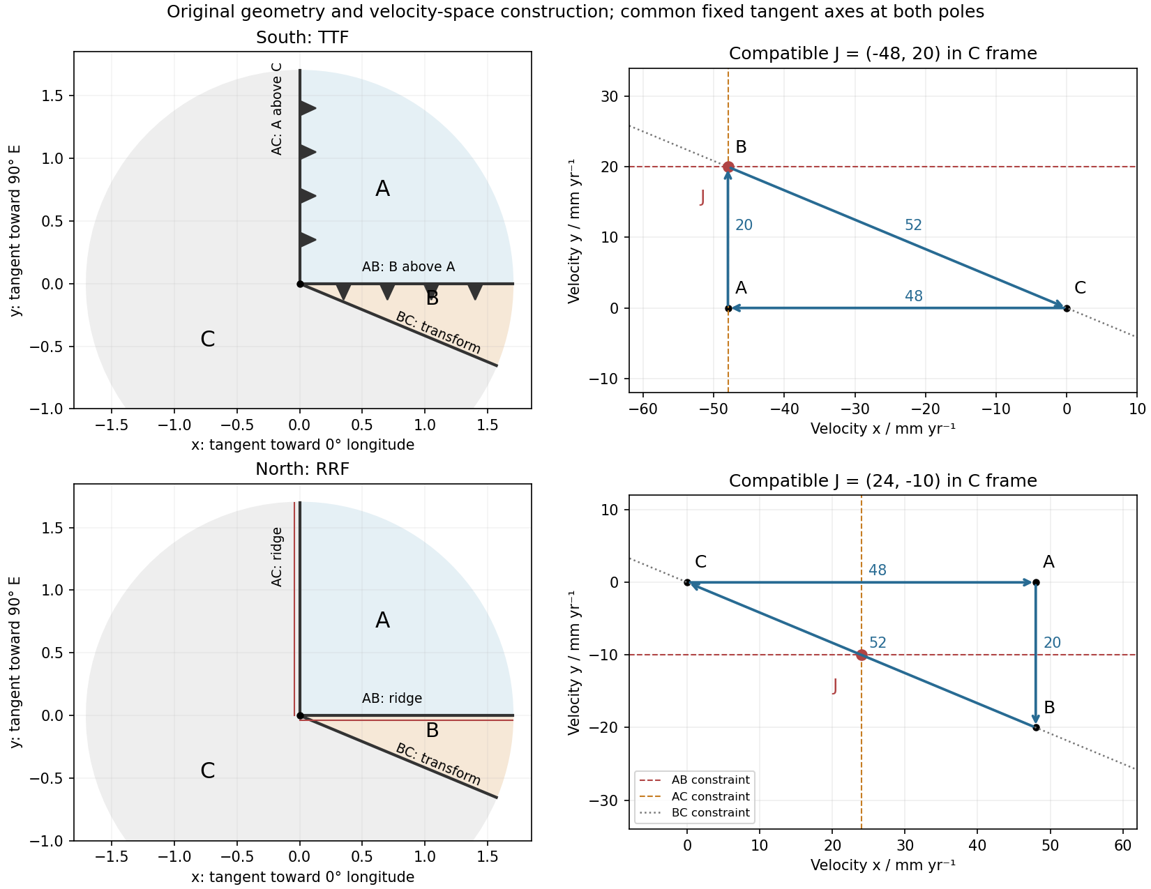
Original polar boundary geometry and plate velocity triangles; dashed velocity-space constraints locate compatible south and north junction velocities
. Details. Past exam of the physics of the Earth as a Planet course of the University of Cambridge 2016 Paper 1 1 b Solution by Codex 0 2026-10-20
Codex 0 2026-10-20At latitude and longitude , . Motion is . A meridian boundary has horizontal normal , so its across-boundary velocity isFor a transform fault this must vanish along the whole meridian, not only at an isolated point. Thus . Select the solution in the western hemisphere:The other solution is the antipodal meridian in the eastern hemisphere. Geometrically, the transform meridian is in a great-circle plane perpendicular to the Euler angular velocity vector. Its outgoing tangent direction at either pole, expressed in the fixed axes, is .
Past exam of the physics of the Earth as a Planet course of the University of Cambridge 2016 Paper 1 1 a Solution by Codex 0 2026-10-20
Codex 0 2026-10-20Let point to the equatorial meridian at zero longitude, to the equator at E, and to the north pole. Use a right-hand positive Euler angular velocity vector. Relative rotations add as vectors, not as geographic coordinates:ConsequentlyHere is the longitude of the positive Euler pole, and its latitude is zero. The antipodal pole with the opposite angular-velocity sign is an equivalent convention; mixing a pole reversal with an unchanged sign would give the wrong motion.
Past exam of the physics of the Earth as a Planet course of the University of Cambridge 2015 Paper 1 3 b Solution by Codex 0 2026-10-20
Codex 0 2026-10-20Homologous temperature and deformation. Homologous temperature is , with both temperatures in kelvin and the appropriate pressure- and composition-dependent melting temperature. It measures proximity to melting more meaningfully than an absolute temperature alone. Pressure, composition and water can alter both and the flow law, so equal does not imply identical rheology.
A useful thermally activated material creep law iswith stress , grain size , activation energy and activation volume . Water activity can add another factor. Increasing temperature raises the rate at fixed stress when the activation enthalpy is positive, greatly lowering effective viscosity. Solid material can therefore flow on geological timescales well below melting.
Diffusion creep is approximately linear in stress: bulk-diffusion Nabarro-Herring creep has grain-size scaling , while grain-boundary Coble creep has in their ideal regimes. Dislocation creep usually has a stress exponent greater than one and weaker grain-size dependence. Its effective viscosity scales as at fixed temperature, so stronger forcing changes the apparent viscosity. At lower homologous temperature, brittle/frictional deformation or high-stress dislocation mechanisms can become important. The dominant process also depends on pressure and confinement; low temperature is not by itself a guarantee of brittle failure deep in a planet.
A deformation mechanism map compares the competing rates or strengths as functions of stress and homologous temperature at specified grain size, pressure and composition. Fine grains favour diffusion creep; larger stress favours nonlinear dislocation creep. There is no universal temperature dividing all these regimes. This sensitivity helps explain a strong outer lithosphere above a slowly flowing solid mantle and why modest thermal or water variations can reorganize deformation.
Determining the actual planform of mantle convection. The task is to infer the geometry of upwellings, downwellings and connecting flow in the present Earth, rather than to draw a preferred laboratory convection cell. Plate velocities and the distribution of subduction zones directly constrain surface motion and likely cold downwellings. Ridges, volcanism and hotspots provide further clues, but a ridge need not mark the centre of a deep plume, nor is every hotspot uniquely explained by one plume geometry.
Seismic tomography supplies three-dimensional velocity structure from body-wave travel times, waveforms and surface-wave dispersion. Fast slab-like structures can often be traced beneath subduction zones into the lower mantle. The 1997 global P-wave study reported long narrow lower-mantle structures connected with convergence and interpreted some slab segments as reaching the deepest mantle; that is evidence for deep circulation, not proof that every slab follows one route.[ref]
Evidence for deep mantle circulation from global tomography by R. D. van der Hilst and others. Nature 386, pages 578–584; abstract on lower-mantle structures and mantle-wide flow
Temperature affects seismic speed, but composition, phase changes, water and anisotropy also matter, so velocity is not itself a flow map.Gravity and the geoid constrain the spatially integrated density field and its induced boundary deformation. Dynamic topography supplies information about vertical stresses, after separating crustal structure, isostatic loads and thermal subsidence. Seismic anisotropy can constrain deformation and fabric orientations, subject to a mineral-physics relation between fabric and flow. Discontinuity topography and the mantle's heat budget provide further tests. Each observation has a different sensitivity to density, temperature and viscosity, making their combination more useful than any one image.
Compare these observations with three-dimensional geodynamic models that solve creeping-flow force balance, mass conservation and thermal transport, including buoyancy from temperature and composition, realistic plate motions, viscosity structure and phase boundaries. Predict seismic observables, gravity, geoid and dynamic topography from the same model, and assess data coverage and resolution before interpreting a feature. Whole-mantle exchange, impeded or deflected slabs near transition zones, and broad deep anomalies can coexist; the evidence does not require identical stacked or single-layer cells everywhere. The actual planform is constrained by joint seismic, gravitational, surface-kinematic and thermal evidence, with substantial nonuniqueness in its detailed flow and history.
Past exam of the physics of the Earth as a Planet course of the University of Cambridge 2015 Paper 1 3 a Solution by Codex 0 2026-10-20
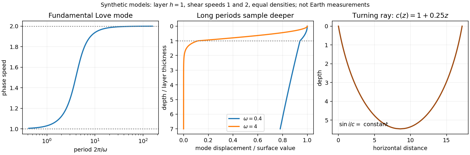
Codex 0 2026-10-20Seismic surface-wave dispersion. Rayleigh waves combine vertical and longitudinal motion in the vertical plane of propagation; Love waves have horizontal transverse motion and can be guided by a low-shear-speed surface layer. A homogeneous elastic half-space supports a Rayleigh wave with a frequency-independent speed in the ideal elastic limit, but depth-dependent Earth structure makes the surface-wave eigenfunctions and their propagation speeds depend on frequency. This structural dispersion can occur even when each constituent material is itself nondispersive.
Distinguish phase velocity from group velocity , which controls a narrow-band envelope in the appropriate weakly attenuating limit. Longer periods generally have deeper sensitivity, while shorter periods emphasize shallower structure. In a profile whose shear speed increases with depth this often makes long-period waves faster, but low-velocity zones, anisotropy and higher modes can change that trend. Frequency dependence need not be monotonic in every Earth model.
Measure phase delays or wave-packet arrival times across known source–receiver paths for many periods, accounting for source phase, cycle ambiguity, multipathing and mode identification. Compute predicted dispersion from trial elastic profiles and compare with observations. Linearization expresses the sensitivity schematically aswhere are compressional and shear speeds. A regularized inverse problem then estimates depth structure; many crossing paths additionally provide surface-wave tomography. Joint Love wave and Rayleigh wave measurements help distinguish shear-wave polarizations and constrain radial seismic anisotropy. Finite bandwidth, depth averaging and correlated sensitivities mean that one dispersion curve does not uniquely determine a detailed Earth profile.
Seismic ray theory, the eikonal equation and Fermat's principle. In a smoothly varying isotropic medium, insert a high-frequency ansatz into the scalar wave equation. The leading powers of frequency giveThe travel-time surfaces are wavefronts and rays are their normal trajectories, with slowness vector . The next-order equation transports amplitude, including geometrical spreading; attenuation is an additional material effect.
Fermat's principle says that the ray makes stationary under path variations with fixed endpoints. Stationarity, rather than always the global minimum, permits multiple arrivals. Its Euler–Lagrange equation, with arclength and unit tangent , isFor horizontal layering, the horizontal slowness is conserved, giving Snell's law at interfaces and smooth refraction between them. Here is measured from vertical. A turning point satisfies ; increasing speed with depth bends a downgoing ray back upwards. Travel-time tomography uses these ray integrals to infer spatial slowness variations.
The approximation requires wavelength to be small compared with structural variation scales. Caustics, turning-point amplitudes, diffraction, scattering and finite-frequency sensitivity require wave-based corrections. Thus seismic ray theory gives an economical geometric description and useful travel times, while surface-wave dispersion retains essential interference and boundary-mode physics.
Past exam of the physics of the Earth as a Planet course of the University of Cambridge 2015 Paper 1 2 d Solution by Codex 0 2026-10-20
Codex 0 2026-10-20Use the supplied surface temperature, , as the premise. With otherwise comparable material and geothermal gradient, this hotter boundary increases thermally activated material creep at shallow depth and places a chosen mechanical cutoff temperature closer to the surface. That effect alone would favour a thinner elastic layer than in a cool terrestrial oceanic plate.
Water weakening of rocks makes dryness act in the opposite direction. Water can enhance material creep; sufficiently dry material can remain strong at temperatures at which its wet equivalent relaxes. Experiments on dry diabase provide a concrete basis for a strong dry crust and possible mechanical coupling between crust and mantle, rather than requiring a weak crustal layer solely because the surface is hot.[ref]
High-temperature deformation of dry diabase, with application to crustal deformation on Venus by S. J. Mackwell and others. 1996, printed pages 793–794, dry strength and implications for crustal coupling
For an illustrative steady conductive geotherm with thermal conductivity and heat flux , a fixed strength cutoff givesTherefore the comparison would scale aswhere all temperatures are compared consistently and a dry rheology may have a higher effective cutoff . This is a conditional strength-layer estimate, not a universal definition of .
Venus can retain appreciable elastic thickness despite its hot surface; temperature favours thinning, while dryness favours strengthening. The supplied facts alone determine neither a numerical nor a definite ordering relative to Earth's oceanic plates. The comparison requires heat flow, subsurface thermal history, material rheology, interior water content and loading timescale. Little atmospheric water is evidence relevant to the hypothesis of dry rocks, not a direct measurement of deep water activity.
Past exam of the physics of the Earth as a Planet course of the University of Cambridge 2015 Paper 1 2 c Solution by Codex 0 2026-10-20
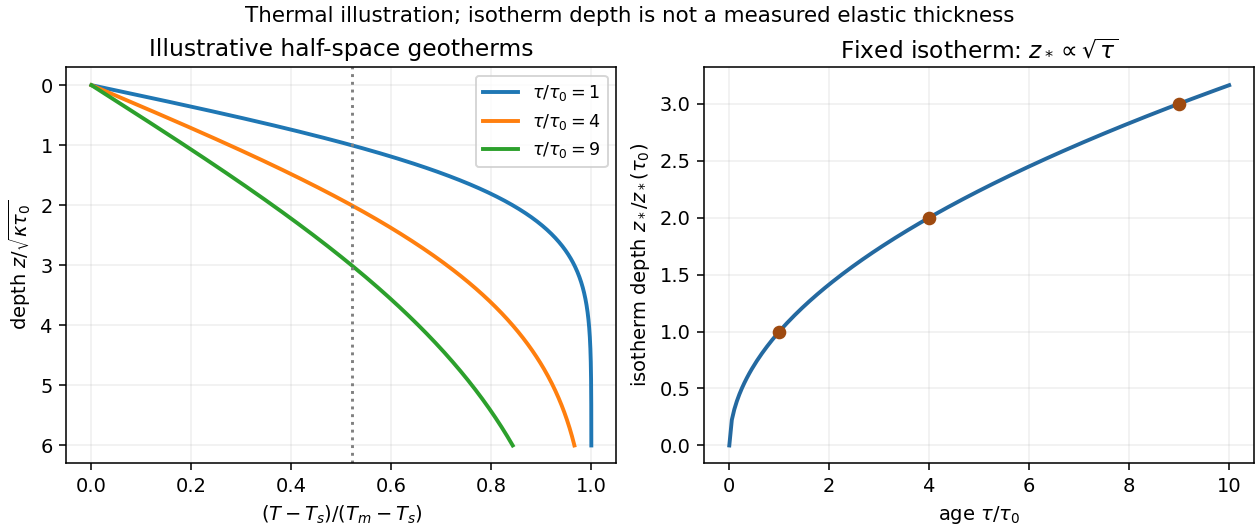
Codex 0 2026-10-20New oceanic lithosphere is hot and mechanically weak. As it cools, the depth over which rock can sustain elastic stress on the loading timescale generally increases, so effective elastic thickness tends to increase with plate age at the time of loading. It is this mechanical state when the load is emplaced, together with subsequent relaxation, that matters; the present age alone is insufficient for an ancient load.
The half-space cooling model illustrates the thermal dependence. With age , surface temperature , initial interior temperature and constant thermal diffusivity ,A chosen temperature lies atIf the base of the mechanically strong layer approximately follows such an isotherm, initially follows a similar age trend. Cooling models constrained by ocean-floor depth and heat flow provide the thermal motivation; their fitted thermal thickness must not be mistaken for measured elastic thickness.[ref]
An analysis of the variation of ocean floor bathymetry and heat flow with age by Barry Parsons and John G. Sclater. 1977, pages 803–806 and discussion of half-space versus finite-plate cooling
In practice is an effective bending thickness rather than the depth of one universal temperature. Stress-dependent yielding, grain size, water content, composition, loading duration and reheating can alter it. Finite-plate cooling and basal heat input also limit indefinite square-root growth at old ages. Nor should be identified with either the thickness of the crust or the full seismically defined lithosphere.
Past exam of the physics of the Earth as a Planet course of the University of Cambridge 2015 Paper 1 2 b Solution by Codex 0 2026-10-20
Codex 0 2026-10-20Define and . ThenAt long wavelength, the mass deficit at the lower interface nearly cancels the surface excess, and the gravity field does not resolve their vertical separation. For ,The first mechanical contribution is fourth order in , although the exponential also contributes terms at second and third order. If the ideal interface depth were zero, the leading term would instead be .
At short wavelength, bending resists the interface's deflection, and any remaining buried signal is attenuated. ConsequentlyThis is the uncompensated surface-sheet value. For nonnegative the approach is from below. With ,The scales and respectively mark gravitational depth filtering and flexural resistance; which appears first depends on . Admittance has dimensions of inverse time squared. The formal limit describes this model, not an assertion that thin-plate theory remains accurate at arbitrarily short wavelength.
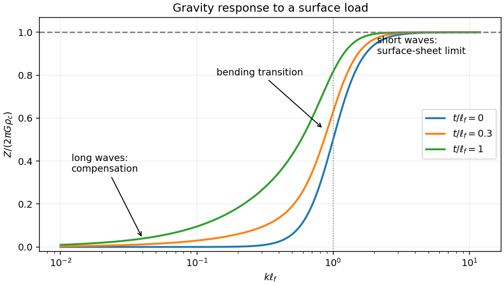
Compensated long wavelengths, flexural transition and the uncompensated gravity limit
. Details. Past exam of the physics of the Earth as a Planet course of the University of Cambridge 2015 Paper 1 2 a Solution by Codex 0 2026-10-20
Codex 0 2026-10-20Take upward deflection as positive, use , and write . A positive added load depresses the plate, so is negative beneath it. Because bending moves the original surface while the load adds thickness, the final topography is . For the cosine mode the horizontal biharmonic operator multiplies by , givingEliminate to obtainThe original loading equation contains , whereas the relation after eliminating the added thickness contains . These must not be interchanged prematurely.
At first order in the relief, represent a displaced density interface by a sinusoidal mass sheet. A sheet of surface-density amplitude at depth produces a downward gravity amplitude at the datum. This follows by solving the Fourier-transformed gravitational Poisson equation above and below the sheet: the decaying potential has amplitude , with the normal derivative jump fixed by the sheet mass.
The top interface contributes ; the displaced crust–mantle interface contributes at depth . ThusThe second term is negative beneath a positive load: depression replaces denser mantle material by lighter crust. Substituting the deflection-to-topography ratio yieldsThis flexural gravity admittance combines mechanical compensation and attenuation of the buried interface's gravitational signal. It assumes small relief, a flat uniform thin plate, uniform density layers and the stated surface loading, without additional internal density anomalies. Here is the depth of the crust–mantle interface. It is not automatically the effective elastic thickness ; the latter enters through .
Past exam of the physics of the Earth as a Planet course of the University of Cambridge 2015 Paper 1 1 c Solution by Codex 0 2026-10-20
Codex 0 2026-10-20For seismic source inversion, collect calibrated, consistently filtered samples from all available stations and components into a data vector . For each trial source position and origin time, compute the corresponding elastodynamic Green tensor in an Earth model, including the instrument response used for the data. Write the symmetric seismic moment tensor in six independent symmetric basis tensors:Each column of is the synthetic seismogram for one basis tensor. An off-diagonal basis tensor contains both symmetric entries, so the double contraction and its factors of two remain consistent.
A suitable objective iswith noise covariance ; a justified penalty can be added for regularization. At fixed , solve for the six entries of by weighted least squares, preferably using a QR decomposition or singular value decomposition rather than explicitly inverting the matrix of the normal equations. Then search over the four nonlinear parameters using a coarse location/time grid followed by local refinement. This variable projection reduces a ten-parameter search to a four-parameter nonlinear search with an inner six-parameter linear fit. Merely having more than ten data samples does not ensure identifiability: the design matrix must have adequate rank and the network must resolve the source's radiation patterns.
Potential errors include inaccurate velocity, density, anisotropy and attenuation in the assumed Earth model; neglected finite rupture and source-time effects; timing, instrument calibration or component-orientation errors; correlated noise; uneven station coverage; and tradeoffs between depth, origin time and the moment tensor. Imposing a double-couple seismic source mechanism without evidence can hide genuine non-double-couple components. Regularization also changes the recovered source and should be reported.
Inspect residuals, singular values, recovery of synthetic sources and uncertainty under resampling or noise perturbations. Linearized covariance or a posterior distribution can quantify uncertainty within the assumed forward model, but does not automatically account for errors in that model. A good waveform fit alone is insufficient evidence that all ten parameters are uniquely recovered.
Past exam of the physics of the Earth as a Planet course of the University of Cambridge 2015 Paper 1 1 a Solution by Codex 0 2026-10-20
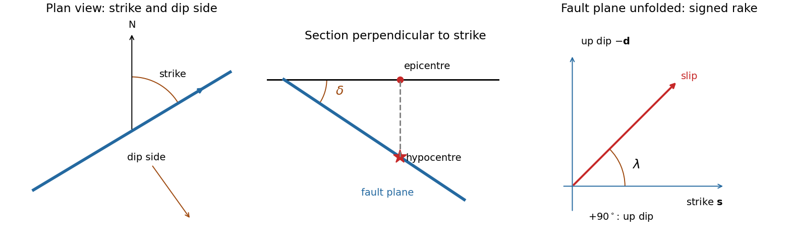
Codex 0 2026-10-20A fault plane represents the surface across which the two sides of a fault slip. A real fault need not be perfectly planar; these angles can describe a local planar segment. Its fault strike is the azimuth, measured clockwise from north, of its horizontal intersection. The line itself has a ambiguity; choose the direction for which the fault dips to the right. Its fault dip, , is the angle below horizontal measured perpendicular to that fault strike, from for horizontal to for vertical.
The fault rake, , is the angle of the relative slip vector within the fault plane. State the sign convention: if is the chosen strike direction and points down dip, useThus is slip along , is up-dip slip and is down-dip slip. This distinguishes the direction in which the fault is tilted from the direction in which it actually moves.
The hypocentre is the point where rupture begins within the Earth. The epicentre is the point on the surface directly above it. The hypocentre need not coincide with the centroid of the final rupture. Orientation uses strike and dip; motion additionally needs rake; epicentre and hypocentre locate the rupture's start.[ref]
Earthquake Hazards Program Glossary by United States Geological Survey. Entries “fault plane”, “strike”, “dip”, “hypocenter” and “epicenter”
Past exam of the physics of the Earth as a Planet course of the University of Cambridge 2014 Paper 1 3 b Solution by Codex 0 2026-10-20
Codex 0 2026-10-20Oceanic thermal subsidence. Newly formed oceanic lithosphere is hot and buoyant. Cooling increases its column density, causing subsidence by isostasy as it moves away from a ridge. The half-space cooling model has profile isWith volumetric thermal expansion coefficient , the excess column mass relative to hot mantle isCompensation with seawater density givesThus young-to-intermediate-age seafloor generally deepens approximately as the square root of age. At old ages, finite thermal-plate thickness and basal heat supply flatten this trend; indefinite half-space deepening is inappropriate. Sediments, variable crust, volcanic swells and dynamic topography also perturb bathymetry. Ocean-floor depth and heat flow jointly constrain cooling models.[ref]
An analysis of the variation of ocean floor bathymetry and heat flow with age by Barry Parsons and John G. Sclater. 1977, half-space cooling, bathymetric age trend and finite-plate alternative
Effective elastic thickness. This is the thickness of a homogeneous elastic plate with the observed effective flexural rigidity, not necessarily the crustal or thermal lithospheric thickness:Infer it by modelling deflection around known loads, such as seamounts or trenches, or fitting gravity-topography admittance and gravity-topography coherence across wavelengths. A simple Fourier balance is for a signed transverse load. The transition from buoyancy-dominated to bending-dominated behaviour constrains ; then assumed Young's modulus and Poisson's ratio give .
Good inference includes load geometry and density, buried interfaces, sediment and internal loading, boundary conditions and data resolution. These can trade off with rigidity. Plastic yielding, faulting, mechanical layering and creep make an effective, timescale- and stress-dependent quantity. Older, colder lithosphere is often stronger, but age at loading and subsequent relaxation matter; a single universal age-to- conversion is unjustified.
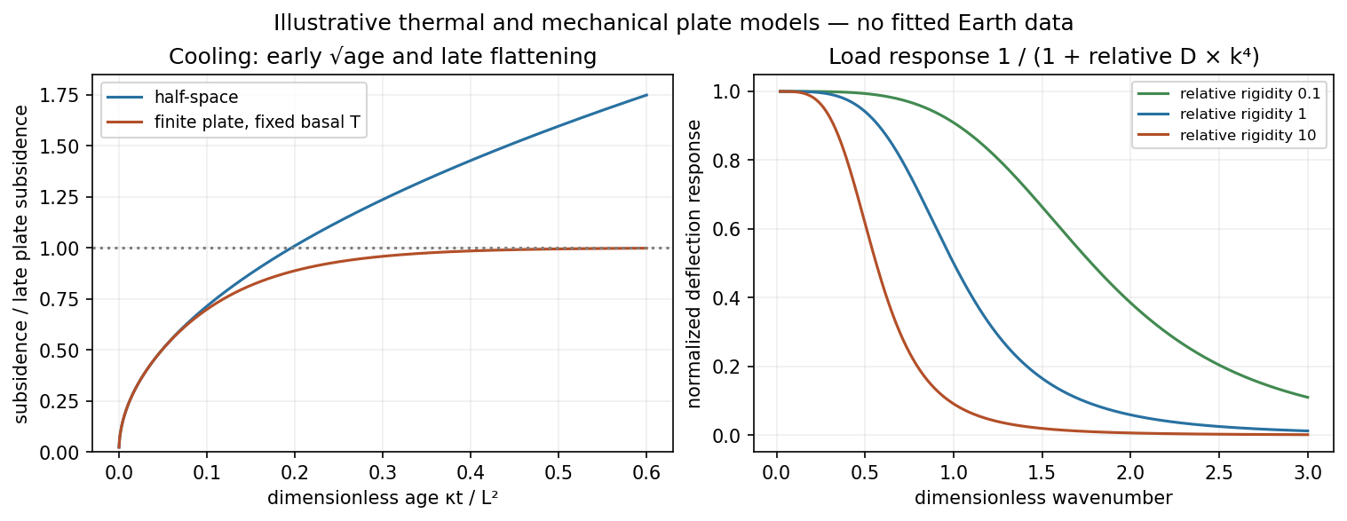
Square-root cooling versus finite-plate saturation, and stiffness sensitivity of the flexural response
. Details. Past exam of the physics of the Earth as a Planet course of the University of Cambridge 2014 Paper 1 3 a Solution by Codex 0 2026-10-20
Codex 0 2026-10-20Elastic rebound. Tectonic motion loads a fault whose shallow portion is locked. Rock on either side deforms and stores elastic strain energy while slip is inhibited. When failure permits rapid slip, part of the stored energy becomes seismic radiation and part is dissipated in friction and damage. The adjacent rock partly relaxes, while a permanent displacement remains across the fault. Geodetic strain accumulation and coseismic offsets support this loading–release picture.[ref]
Reid's Elastic Rebound Theory by United States Geological Survey. Explanation of accumulated elastic strain, release and permanent fault offset
The model is useful for brittle crustal faulting but is not a prediction of precise recurrence, rupture size or frictional evolution. Aseismic creep can release deformation without a large sudden event. Viscoelastic flow, afterslip, fluid-pressure changes and interacting fault segments complicate a simple locked-fault cycle. Deep-focus earthquakes and non-shear source components require additional physics; not every earthquake source is adequately described by a shallow brittle double couple. Rebound also need not release all the pre-existing stress.
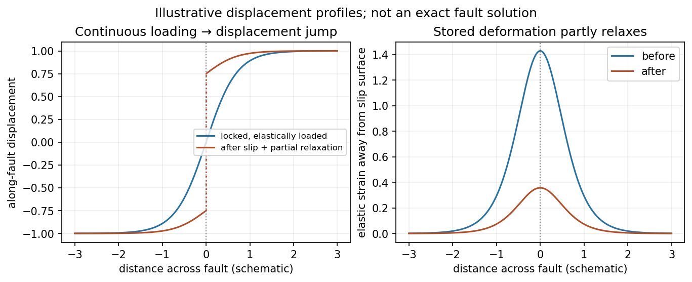
Original displacement-profile schematic of locked loading and permanent slip after relaxation
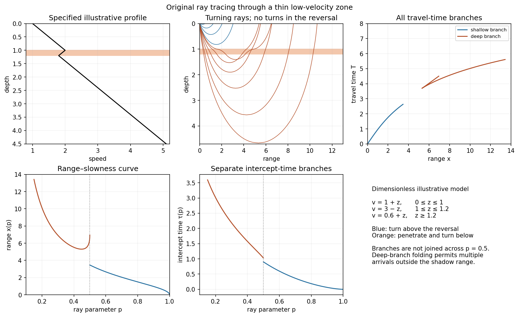
. Details. A thin negative-gradient velocity zone. In horizontal layering, use the seismic ray parameter , the conserved horizontal slowness. A ray turns when . Downward passage through decreasing speed makes smaller, so a surface ray cannot turn in the negative-gradient interior. Rays either turn above the zone or penetrate it and turn below where speed has recovered sufficiently. This produces missing turning depths and a seismic shadow range from a low-velocity zone in the ideal ray model.
Retain all branches usingThe travel-time slope is . Just below the critical value that permits passage beyond the upper speed maximum, the ray makes a finite extra excursion through the low-velocity region. Range can jump, and the deep branch can fold back before resuming its normal trend, giving multiple arrivals outside the shadow. A first-arrival curve alone hides some of these branches. Define the seismic intercept time byThe – representation displays the gap and fold; the – representation has separate shallow and deep branches and a branch jump at the critical ray parameter for the piecewise-linear cusp model. Do not join them by invented turning rays. Diffraction and finite-frequency energy soften a purely geometrical shadow.
The figures use an explicit illustrative profile, not measured Earth parameters: speed rises from 1 to 2 over depths 0 to 1, falls to 1.8 by depth 1.2, then rises with its original gradient. The asthenosphere beneath oceanic lithosphere is an important setting for a low-velocity zone. A major P-wave speed reduction also occurs at the boundary between the mantle and the outer core of the Earth; S waves do not propagate through the liquid outer core of the Earth.[ref]
Essentials of Geophysics: Seismology by R. D. van der Hilst. Chapter 4, printed pages 169–170, low-velocity-zone rays, shadow range and Earth examples
Pinned article: Introduction to the OurBigBook Project
Welcome to the OurBigBook Project! Our goal is to create the perfect publishing platform for STEM subjects, and get university-level students to write the best free STEM tutorials ever.
Everyone is welcome to create an account and play with the site: ourbigbook.com/go/register. We belive that students themselves can write amazing tutorials, but teachers are welcome too. You can write about anything you want, it doesn't have to be STEM or even educational. Silly test content is very welcome and you won't be penalized in any way. Just keep it legal!
Intro to OurBigBook
. Source. We have two killer features:
- topics: topics group articles by different users with the same title, e.g. here is the topic for the "Fundamental Theorem of Calculus" ourbigbook.com/go/topic/fundamental-theorem-of-calculusArticles of different users are sorted by upvote within each article page. This feature is a bit like:
- a Wikipedia where each user can have their own version of each article
- a Q&A website like Stack Overflow, where multiple people can give their views on a given topic, and the best ones are sorted by upvote. Except you don't need to wait for someone to ask first, and any topic goes, no matter how narrow or broad
This feature makes it possible for readers to find better explanations of any topic created by other writers. And it allows writers to create an explanation in a place that readers might actually find it.
Figure 1. Screenshot of the "Derivative" topic page. View it live at: ourbigbook.com/go/topic/derivativeVideo 2. OurBigBook Web topics demo. Source. - local editing: you can store all your personal knowledge base content locally in a plaintext markup format that can be edited locally and published either:This way you can be sure that even if OurBigBook.com were to go down one day (which we have no plans to do as it is quite cheap to host!), your content will still be perfectly readable as a static site.
- to OurBigBook.com to get awesome multi-user features like topics and likes
- as HTML files to a static website, which you can host yourself for free on many external providers like GitHub Pages, and remain in full control

Figure 2. You can publish local OurBigBook lightweight markup files to either OurBigBook.com or as a static website.
Figure 3. Visual Studio Code extension installation.
Figure 5. . You can also edit articles on the Web editor without installing anything locally. Video 3. Edit locally and publish demo. Source. This shows editing OurBigBook Markup and publishing it using the Visual Studio Code extension. 
- Infinitely deep tables of contents:




All our software is open source and hosted at: github.com/ourbigbook/ourbigbook
Further documentation can be found at: docs.ourbigbook.com
Feel free to reach our to us for any help or suggestions: docs.ourbigbook.com/#contact