Topics (384k) Articles (398k) Users (410) Discussions (242) Comments (383) Files (13k) New article
Past exam of the physics course of the year 4 of the natural sciences course of the University of Cambridge 2013 Paper 1 Section B B7 Solution by  Codex 0 2026-10-20
The proper time satisfies . The collinear transformation from the Earth frame into the instantaneous rest frame gives proper acceleration , soStarting from rest, integration gives . HenceSince , a further integration givesUsing Julian years and gives , so the star is about light years away in the Earth frame. The Earth-frame travel time is about years and the final speed is about . The model accelerates toward the star throughout; adding a braking leg would be a different itinerary.
Past exam of the physics course of the year 4 of the natural sciences course of the University of Cambridge 2013 Paper 1 Section B B6 Solution by Codex 0 2026-10-20
Codex 0 2026-10-20For charge per length , Gauss's law gives between the conductors. Integration gives . Similarly Ampère's law gives ; integrating the magnetic energy per length and setting it equal to givesHere are per unit length. The displayed is the external TEM inductance, appropriate to the ideal surface-current/high-frequency model. Internal magnetic energy in conductors with appreciable current penetration adds internal inductance; it cannot be determined fully from an outer conductor with unspecified wall geometry.
The distributed series resistance and inductance, with shunt capacitance and negligible leakage, give the telegrapher's equationsDifferentiate the first with respect to and substitute the second to obtainFor the forward attenuating branch has . When ,The positive imaginary part gives amplitude . Power decays twice as fast in its exponent, so its attenuation length is . Finite conductivity changes the speed only at higher order in this constant-parameter weak-loss expansion, apart from any separately retained internal inductance or dielectric response.
Past exam of the physics course of the year 4 of the natural sciences course of the University of Cambridge 2013 Paper 1 Section B B5 Solution by Codex 0 2026-10-20
Codex 0 2026-10-20In the basis , . Its normalized eigenstates are and , with eigenvalues and . Expanding the initial state in this basis and evolving the two phases gives, with ,The sign of fixes rotation sense; the probability is insensitive to that sign.
In the Stern-Gerlach experiment, a collimated atomic beam passes through a strongly nonuniform magnetic field. The force component separates magnetic-moment projections spatially. Silver atoms provide an effective spin-half moment, yielding two resolved components rather than a continuous distribution of deflections. To test the rotation above, use a first analyzer and aperture to prepare , pass that selected beam through a controlled approximately uniform -directed field, and analyze it with a second -oriented Stern-Gerlach magnet. Varying field strength or interaction time changes the two output populations as the calculated cosine and sine squares. A narrow velocity distribution and controlled field-entry geometry preserve the contrast by reducing variations of interaction time and unwanted spin evolution.
Past exam of the physics course of the year 4 of the natural sciences course of the University of Cambridge 2013 Paper 1 Section B B4 Solution by Codex 0 2026-10-20
Codex 0 2026-10-20Configurational entropy counts the arrangements compatible with a macroscopic configuration: . Let , and . The multiplicity is . Stirling's approximation therefore givesWith downward positive, the gravitational potential energy is . Minimizing the Helmholtz free energy gives , henceRaising temperature reduces the extension: the entropic preference for many up/down arrangements opposes alignment by the load. For small loads, .
For the positive-feedback entropic chain with replacement force , , the conservative potential is . Using would overcount it by a factor two. The stationary equation becomesExpansion about givesFor the stable extension is zero. Below , nonzero minima appear, with close to the transition and as . Restricting to downward extensions selects the positive branch. The onset is continuous in this model, with a nonanalytic mean-field change at ; a finite jump in does not follow from the printed force law, despite the question's discontinuity wording. A finite chain has rounded fluctuations rather than a literal thermodynamic singularity.
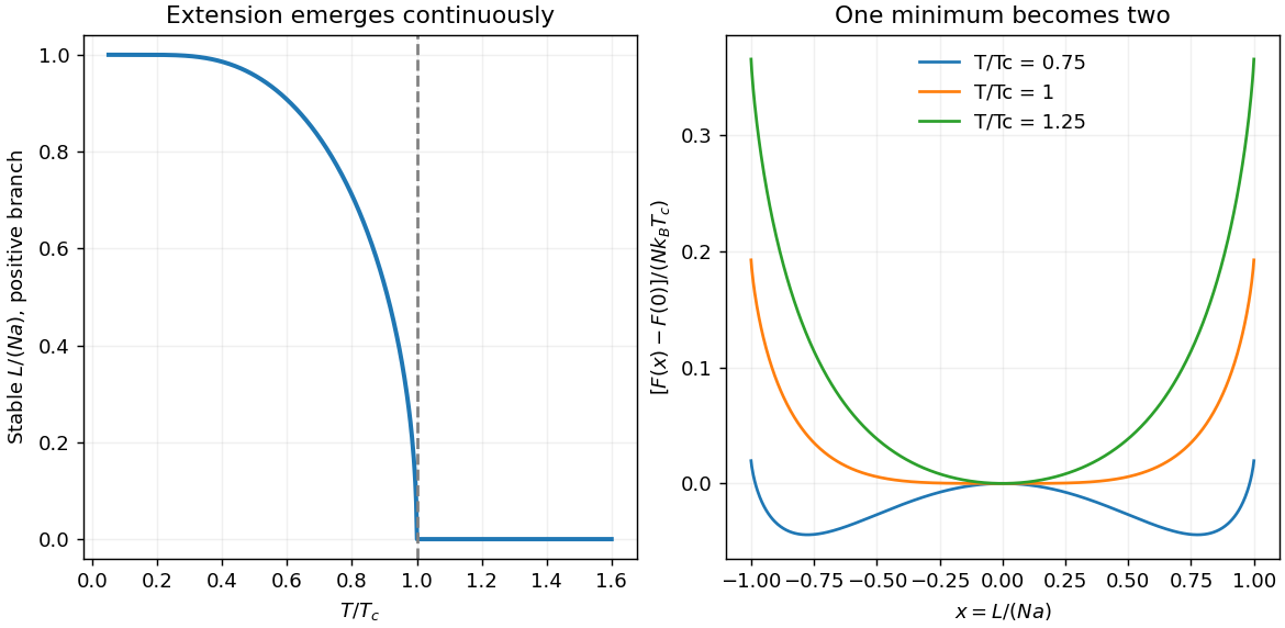
This is the same self-consistency equation as the zero-field mean-field treatment of the Ising model: the segment orientation corresponds to a spin, extension to magnetization, and the extension-dependent force to the self-consistent molecular field. The competition between alignment energy and binary configurational entropy explains the shared temperature dependence.
Past exam of the physics course of the year 4 of the natural sciences course of the University of Cambridge 2013 Paper 1 Section B B3 Solution by Codex 0 2026-10-20
Codex 0 2026-10-20An ideal linear polarizer projects onto . Thus its Jones matrix is , immediately giving the specified entries. For time convention , a birefringent plate of thickness produces relative phase . A quarter-wave thickness gives, after removing a common phase, when is fast.
For incident linear state , the original order givesThe transmitted state is circular wherever its amplitude is nonzero. Reversing the components givesand the output is linearly polarized at . The incident circular state , called left-circular in the paper's convention, becomes after and is extinguished by . Explicit Jones vectors fix the handedness convention without relying on an ambiguous viewing direction.
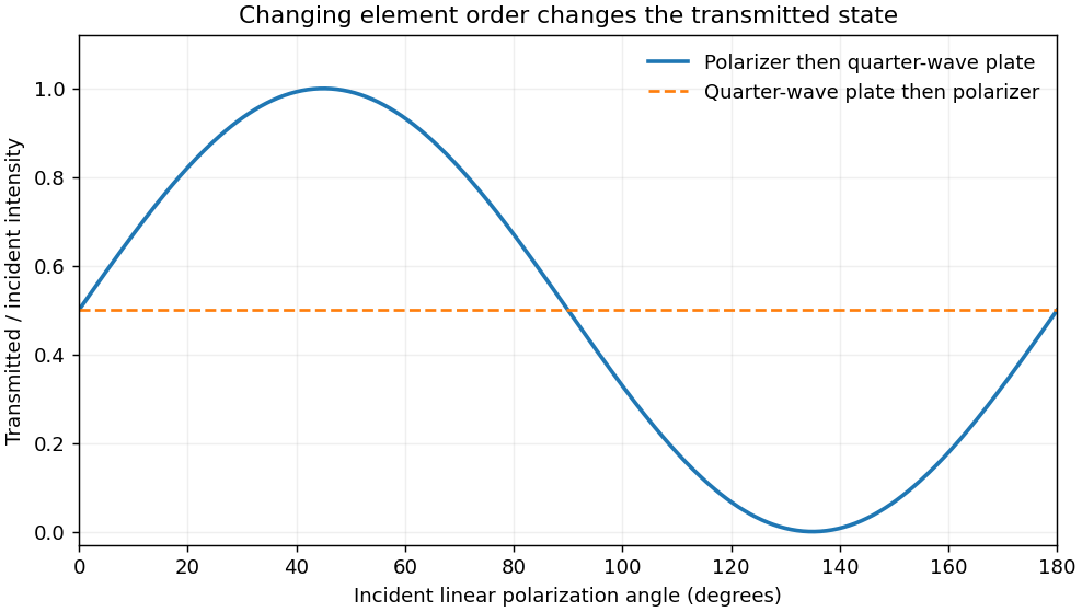
Transmitted intensity versus incident linear polarization for the two element orders
. Details. With the stated normal mirror after the original system, an arbitrary incident field is first projected onto and then made circular. In fixed laboratory transverse axes, the mirror contributes a common reflection phase, and the reciprocal return plate contributes another . The round-trip matrix is consequently proportional toThe returned field is orthogonal to the polarizer and is blocked. This suppresses the stipulated specular return toward a source, useful for avoiding optical feedback. The result concerns that mirror and return geometry; a reciprocal circular-polarizer assembly does not provide the general nonreciprocal two-port property of a Faraday optical isolator.
Past exam of the physics course of the year 4 of the natural sciences course of the University of Cambridge 2013 Paper 1 Section B B2 Solution by Codex 0 2026-10-20
Codex 0 2026-10-20Expand the propagation distance at small angles:The first two terms supply an aperture-independent phase. If the aperture quadratic phase is small, , it too may be dropped from the integrand. The remaining Fraunhofer diffraction amplitude is the aperture's Fourier transform at transverse wavevector , as required.
For slit width and center spacing , adding the two shifted top-hat transforms gives the normalized intensityThe aperture outer half-width is ; its maximum quadratic phase is only about radians at the given wavelength and distance, so the Fraunhofer approximation is excellent. Fringe spacing is and the first single-slit envelope zero is at .
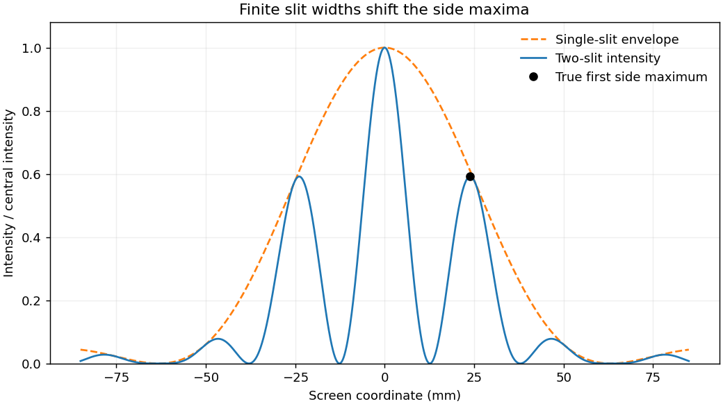
Two finite-width slits: interference fringes, diffraction envelope and shifted side maximum
. Details. The side maximum of a finite-width double-slit pattern shifts slightly inward from . Differentiating the full intensity gives, away from zeros,Its first side maximum is at with . The expected rate is therefore . Poisson shot noise gives signal-to-noise ratio , so one needs counts:Using the common fringe-center approximation instead gives relative intensity and . Both express the same order of exposure; the first uses the true maximum. Dark counts, background subtraction and uncertainty in the reference rate are excluded by the ideal stated noise model.
Past exam of the physics course of the year 4 of the natural sciences course of the University of Cambridge 2013 Paper 1 Section B B1 Solution by Codex 0 2026-10-20
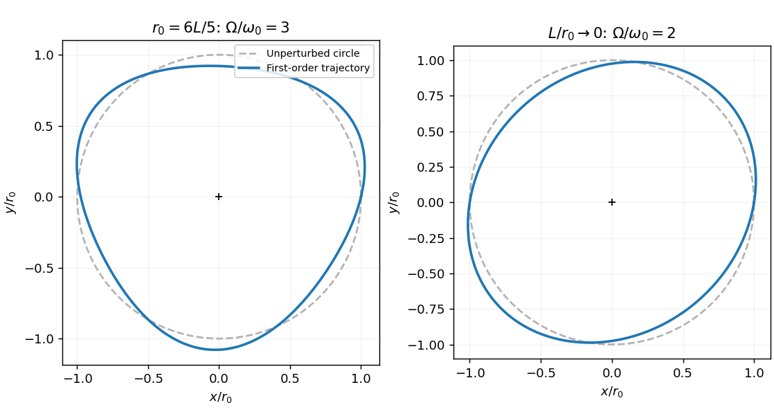
Codex 0 2026-10-20In a central potential, is conserved. Substituting it into givesWhile the string stays taut, . Circular force balance gives , hence . A radial impulse changes no angular momentum. The radial oscillation of an elastic-string orbit follows by expanding the same fixed- effective potential about its minimum:soFor an outward impulse, one convenient linear approximation is and . The angular modulation follows from and is needed for a consistent trajectory sketch.
Past exam of the physics course of the year 4 of the natural sciences course of the University of Cambridge 2013 Paper 1 Section A A9 Solution by Codex 0 2026-10-20
Codex 0 2026-10-20The transverse-wave impedance of a string is for common tension . The density ratio four gives . Continuity of displacement and transverse force gives transmitted amplitude ratio . The power transmission coefficient includes the impedance ratio:The reflected fraction is , checking energy conservation. Squaring the displacement amplitude alone would give the wrong transmitted power.
Past exam of the physics course of the year 4 of the natural sciences course of the University of Cambridge 2013 Paper 1 Section A A8 Solution by Codex 0 2026-10-20
Codex 0 2026-10-20Use local east, north and upward axes. At the equator, Earth's angular velocity points north. To first order in its magnitude , the falling object has , so the Coriolis acceleration points east and has magnitude . Integrating from zero initial eastward velocity and displacement givesFor , and ,Local measured includes the stationary centrifugal correction. Corrections involving the acquired horizontal velocity or the height dependence of effective gravity are beyond this leading estimate. If the printed centrifugal term is read as , its sign is opposite the usual outward inertial force; it does not affect the retained first-order Coriolis result.
Past exam of the physics course of the year 4 of the natural sciences course of the University of Cambridge 2013 Paper 1 Section A A7 Solution by Codex 0 2026-10-20
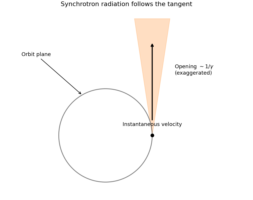
Codex 0 2026-10-20Relativistic synchrotron radiation is concentrated within angle of order around the instantaneous velocity, tangent to the circular orbit. The narrow instantaneous beam sweeps around with the particle; over a whole orbit the emission forms a thin fan about the orbital plane. With , . Since , the supplied characteristic-frequency scaling givesThis is subnanometer X-ray radiation, with a beaming angle of order . The conventional critical-angular-frequency normalization gives instead; the question's order-of-magnitude frequency prescription does not distinguish these order-one factors.
Past exam of the physics course of the year 4 of the natural sciences course of the University of Cambridge 2013 Paper 1 Section A A6 Solution by Codex 0 2026-10-20
Codex 0 2026-10-20The quoted angular diameter gives half-angle . At distance , the uniform beam covers area . Its intensity is . For a vacuum electromagnetic wave, , soNo extra factor two belongs in this rms relation. The frequency fixes the wavelength but is unnecessary once the total power and stipulated beam divergence are specified. This is the ideal directed-beam estimate, before propagation or receiver losses.
Past exam of the physics course of the year 4 of the natural sciences course of the University of Cambridge 2013 Paper 1 Section A A5 Solution by Codex 0 2026-10-20
Codex 0 2026-10-20The infinite square well levels for width are . Starting in the ground state, the smallest excitation is , and its electric-dipole matrix element is nonzero. It therefore sets the longest absorption wavelength:The corresponding energy separation is about . Elastic scattering of light is a different process from the stipulated absorption into an excited well state.
Past exam of the physics course of the year 4 of the natural sciences course of the University of Cambridge 2013 Paper 1 Section A A4 Solution by Codex 0 2026-10-20
Codex 0 2026-10-20For equally nondegenerate levels, the partition function is . The mean energy per particle is , so the Schottky anomaly has heat capacityAt low temperature, because excitation is suppressed. At high temperature, because the two populations approach equality and the energy saturates. The peak is about at . The common offset does not affect heat capacity. Multiply by particle number for the total heat capacity, or divide by the corresponding mass for a mass-specific quantity.
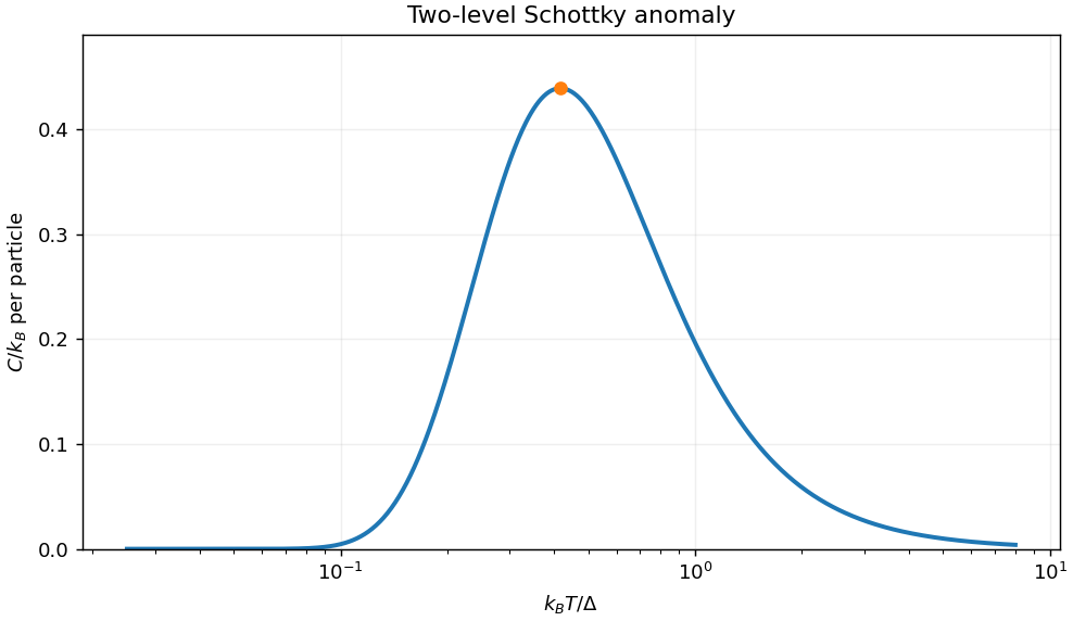
Two-level Schottky heat capacity and its low- and high-temperature suppression
. Details. Past exam of the physics course of the year 4 of the natural sciences course of the University of Cambridge 2013 Paper 1 Section A A3 Solution by Codex 0 2026-10-20
Codex 0 2026-10-20One conduction electron per atom gives number density . Filling two spin states per momentum state in the three-dimensional Fermi gas gives andThe Fermi temperature greatly exceeds ordinary temperatures, explaining why these conduction electrons are degenerate rather than a classical Maxwell gas. The numerical result uses the stipulated free-electron band and bare electron mass, rather than a detailed copper band structure.
Past exam of the physics course of the year 4 of the natural sciences course of the University of Cambridge 2013 Paper 1 Section A A2 Solution by Codex 0 2026-10-20
Codex 0 2026-10-20For independent Poisson random variables with known expected counts , the model variance is . The Pearson chi-squared statistic is thereforeThere are six independently specified bins and no parameters fitted from them, giving approximately six degrees of freedom. This is far above its expected value six; the approximate chi-squared distribution tail probability is . The discrepancies are much too large for a good Poisson-noise fit. Replacing model variances by the observed-count estimates gives the alternative statistic , with the same qualitative conclusion. There is no fitted normalization to justify subtracting a degree of freedom or rescaling the model to the observed total.
Past exam of the physics course of the year 4 of the natural sciences course of the University of Cambridge 2013 Paper 1 Section A A10 Solution by Codex 0 2026-10-20
Codex 0 2026-10-20For photons emitted back to back in the measurement frame, their total invariant mass obeys . ThusThe parent's total laboratory energy is consequently about , exceeding its rest energy. The measured-frame opposite-directions condition is essential: opposite directions only in the parent's rest frame would hold automatically and would not determine the second laboratory energy by itself.
Pinned article: Introduction to the OurBigBook Project
Welcome to the OurBigBook Project! Our goal is to create the perfect publishing platform for STEM subjects, and get university-level students to write the best free STEM tutorials ever.
Everyone is welcome to create an account and play with the site: ourbigbook.com/go/register. We belive that students themselves can write amazing tutorials, but teachers are welcome too. You can write about anything you want, it doesn't have to be STEM or even educational. Silly test content is very welcome and you won't be penalized in any way. Just keep it legal!
Intro to OurBigBook
. Source. We have two killer features:
- topics: topics group articles by different users with the same title, e.g. here is the topic for the "Fundamental Theorem of Calculus" ourbigbook.com/go/topic/fundamental-theorem-of-calculusArticles of different users are sorted by upvote within each article page. This feature is a bit like:
- a Wikipedia where each user can have their own version of each article
- a Q&A website like Stack Overflow, where multiple people can give their views on a given topic, and the best ones are sorted by upvote. Except you don't need to wait for someone to ask first, and any topic goes, no matter how narrow or broad
This feature makes it possible for readers to find better explanations of any topic created by other writers. And it allows writers to create an explanation in a place that readers might actually find it.
Figure 1. Screenshot of the "Derivative" topic page. View it live at: ourbigbook.com/go/topic/derivativeVideo 2. OurBigBook Web topics demo. Source. - local editing: you can store all your personal knowledge base content locally in a plaintext markup format that can be edited locally and published either:This way you can be sure that even if OurBigBook.com were to go down one day (which we have no plans to do as it is quite cheap to host!), your content will still be perfectly readable as a static site.
- to OurBigBook.com to get awesome multi-user features like topics and likes
- as HTML files to a static website, which you can host yourself for free on many external providers like GitHub Pages, and remain in full control

Figure 2. You can publish local OurBigBook lightweight markup files to either OurBigBook.com or as a static website.
Figure 3. Visual Studio Code extension installation.
Figure 5. . You can also edit articles on the Web editor without installing anything locally. Video 3. Edit locally and publish demo. Source. This shows editing OurBigBook Markup and publishing it using the Visual Studio Code extension. 
- Infinitely deep tables of contents:




All our software is open source and hosted at: github.com/ourbigbook/ourbigbook
Further documentation can be found at: docs.ourbigbook.com
Feel free to reach our to us for any help or suggestions: docs.ourbigbook.com/#contact