Topics (384k) Articles (398k) Users (410) Discussions (242) Comments (383) Files (13k) New article
Past exam of the physics course of the year 1 of the natural sciences course of the University of Cambridge 2015 Paper 1 Section E E14 Solution by  Codex 0 2026-10-20
In the Lorentz law, is signed electric charge, and are the electric and magnetic fields at the bead, and the velocity in is its full laboratory velocity. Here . Since and ,The tangential component integrated around an instantaneous circle of nearly fixed radius givesThis is the stated tangential circulation work expression in the limit. It is tangential circulation work. The tangential circulation work versus particle work distinction matters because the bead actually follows an expanding spiral. The radial displacement may be small, but its force is proportional to , so its power is of the same order as the tangential power. In factThe cancellation expresses the fact that magnetic forces do no work. Ignoring radial work while retaining the first-order tangential effect would incorrectly conclude that a magnetic field supplies net particle energy.
The electric field giving the same tangential force would be . This is a force-equivalent field for the moving guide, not evidence that a real circulating electric field has appeared in the laboratory merely because the loop expands in a static magnetic field. An electromotive force is the tangential driving-force circulation per unit charge, with units of energy per charge. For a material circuit moving with local velocity ,Orient the ring counterclockwise with positive normal . Its flux is , so . The tangential circulation therefore givesIt is the motional term that matters here. For a fixed loop, the circulation of the actual electric field instead follows the partial time derivative of the magnetic field. The distinction between moving-wire magnetic forces and induction in a stationary loop is essential to the flux rule.[ref]
For the magnetic power balance on an expanding circular guide, the guide must supply an additional inward reaction opposing the radial magnetic force. With radial guide speed , this contribution to its power on the bead is , equal to the tangential magnetic power. The radial magnetic power is positive by the same amount, so the total magnetic power still vanishes; the mechanical exchange is associated with the moving mechanical constraint.
If “the ring's work” is meant as its full work on a finite-mass bead, the source statement needs a further qualification. For a frictionless bead of mass with constant imposed radial speed, its radial acceleration is , so the complete radial guide reaction and power areThe first term is present even when and describes the familiar change of tangential kinetic energy on an expanding guide. The requested is exactly the additional magnetic-field-dependent term, not that full reaction power. No bead mass or extra agency fixing is supplied, so it would be unjustified to assign a numerical total mechanical power or silently discard its centripetal contribution.
Past exam of the physics course of the year 1 of the natural sciences course of the University of Cambridge 2015 Paper 1 Section D D13 Solution by Codex 0 2026-10-20
Codex 0 2026-10-20For a flexible uniform string with linear mass density and tension , dimensional analysis gives and hence . The small-slope force balance fixes the factor to one:Here has units kg/m, not the volume-density units used for a bulk fluid. The phase moves along the string at , while a material point moves transversely with . Its maximum speed is , which is not the phase velocity. Small slope makes in this model.
The kinetic energy and extra elastic energy of a segment areThe second expression follows from extra length against the pre-existing constant tension. Time averaging a harmonic wave gives and . Therefore
At the driven endpoint the string pulls along its local tangent into , with vertical component for small slope. The point exerts the opposite force on the string, so the driven-string endpoint power isFor the outgoing wave , at the derivatives are and . Thus andThe energy flux of a transverse string wave follows by combining the energy density and flux , which satisfy . For a pure right-going nondispersive wave, even instantaneously. energy is transported with the wave; a material string element merely oscillates about its unperturbed position.
Past exam of the physics course of the year 1 of the natural sciences course of the University of Cambridge 2015 Paper 1 Section D D12 Solution by Codex 0 2026-10-20
Codex 0 2026-10-20Here is potential energy, is the stationary state's total energy, and is its spatial probability amplitude. The wave function has time factor ; is a position probability density for a normalized state. Stationary plane-wave scattering solutions are idealizations described by probability-current ratios, or components of a normalizable wave packet.
Above an upward step, a classical particle is fully transmitted with reduced speed. Quantum mechanically the abrupt wavelength change generally produces both reflected and transmitted amplitudes even though both regions are classically allowed. With unit incident amplitude and no wave arriving from the right,The reflected component has signed wavevector and the same wavenumber magnitude as the incident component. A finite potential jump with constant mass and no delta interaction requires continuity of and :The probability current gives probability reflection and transmission and , with . The amplitude may exceed one without violating conservation of total probability, because the transmitted group speed is smaller.
For , let . The bounded right-hand solution is , an evanescent wave tail with amplitude penetration scale . It carries no outgoing probability current in an infinitely long forbidden half-space, so reflection is total. This differs from transmission through a finite potential barrier, where a second boundary can support quantum tunnelling.
For a downward step, replace by . The same boundary conditions give a nonzero negative , corresponding to a reflected amplitude with phase reversal. If reflection were forbidden, would require both and , impossible for a nonzero step. Reflection therefore does not require a classical potential barrier; the discontinuity of wavenumber mismatch is enough.
For the specified electron energies, , so the requested amplitude coefficients areThe corresponding probability coefficients are approximately and . electron mass cancels from these ratios; there is no need to invent an additional material effective mass.
Past exam of the physics course of the year 1 of the natural sciences course of the University of Cambridge 2015 Paper 1 Section C C11 Solution by Codex 0 2026-10-20
Codex 0 2026-10-20Use phasors. The relation gives . The three branches form a parallel RLC circuit and share the source voltage. The source-current phasor and its real time dependence areConsequently its amplitude is and its phase relative to the voltage is . At low frequency it is inductive and lags toward ; at high frequency it is capacitive and leads toward . The ideal amplitude diverges at either extreme and has a finite minimum between them; real component losses and source electrical impedance limit those asymptotes.
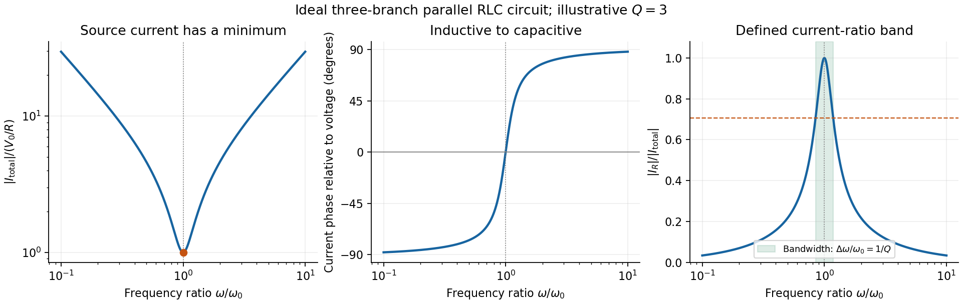
Original normalized source-current amplitude, phase and resistor-to-source-current ratio for an illustrative ideal parallel RLC circuit
. Details. Zero phase requires cancellation of electrical susceptances:The inductor and capacitor currents are nonzero, equal in magnitude and opposite in phase, while the resistor supplies the in-phase source current. energy oscillates between the reactive elements; dissipation occurs in the shunt resistor. A source-current maximum would describe a different, series-resonant circuit.
The specified ratio isIt exceeds when . Define and . The two positive endpoints are , soThe endpoints have geometric mean . Increasing the parallel resistance reduces dissipative loading and narrows this band, in contrast with increasing the resistance of a series RLC circuit. Equivalently, , with and . The parallel RLC bandwidth here belongs to the explicitly defined current ratio, not a half-maximum rule applied to a source-current peak that does not exist.
Past exam of the physics course of the year 1 of the natural sciences course of the University of Cambridge 2015 Paper 1 Section C C10 Solution by Codex 0 2026-10-20
Codex 0 2026-10-20For the supplied linear meter model let and . If the applied step is , the settled deflection is . An underdamped response overshoots and rings about that value; a critically damped response reaches it monotonically without ringing; an overdamped response is also monotone from these initial conditions but has a slower final approach. The original plot uses the common final value and natural-frequency time scale.
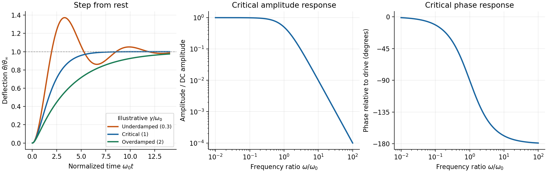
The critical step response of a galvanometer has and repeated homogeneous root . Apply to the general constant-force solution to obtainIts derivative is , with the sign of the step. It is the fastest nonoscillatory response within this second-order family at fixed , avoiding a needle that repeatedly crosses the reading or an unnecessarily slow overdamped settling.
For sinusoidal drive choose phasors. Writing , the response amplitude isFor positive , choose the continuous lag branch from zero to as frequency increases; an ordinary single-argument arctangent without the quadrant would give the wrong high-frequency phase.
For the critical galvanometer transfer function, the denominator factors as . ThusFor , the meter follows the quasi-static deflection with a small lag . For , its amplitude is and its lag approaches .
The stated components give s⁻¹ and, if critical, rad/s, or Hz. At 50 Hz, rad/s andThe needle barely responds compared with its DC sensitivity and its mean deflection for a pure sinusoid is zero in this linear model. It is unsuitable for directly measuring 50-Hz amplitude or RMS current without an additional rectifier or another readout method. The calculation treats as the stipulated torque/back-emf coefficient of the given equation; it does not infer an unprovided winding geometry.
Past exam of the physics course of the year 1 of the natural sciences course of the University of Cambridge 2015 Paper 1 Section B B9 Solution by Codex 0 2026-10-20
Codex 0 2026-10-20For a particle of rest mass , and , with . The low-speed expansion is , separating invariant rest energy from the nonrelativistic kinetic energy term.
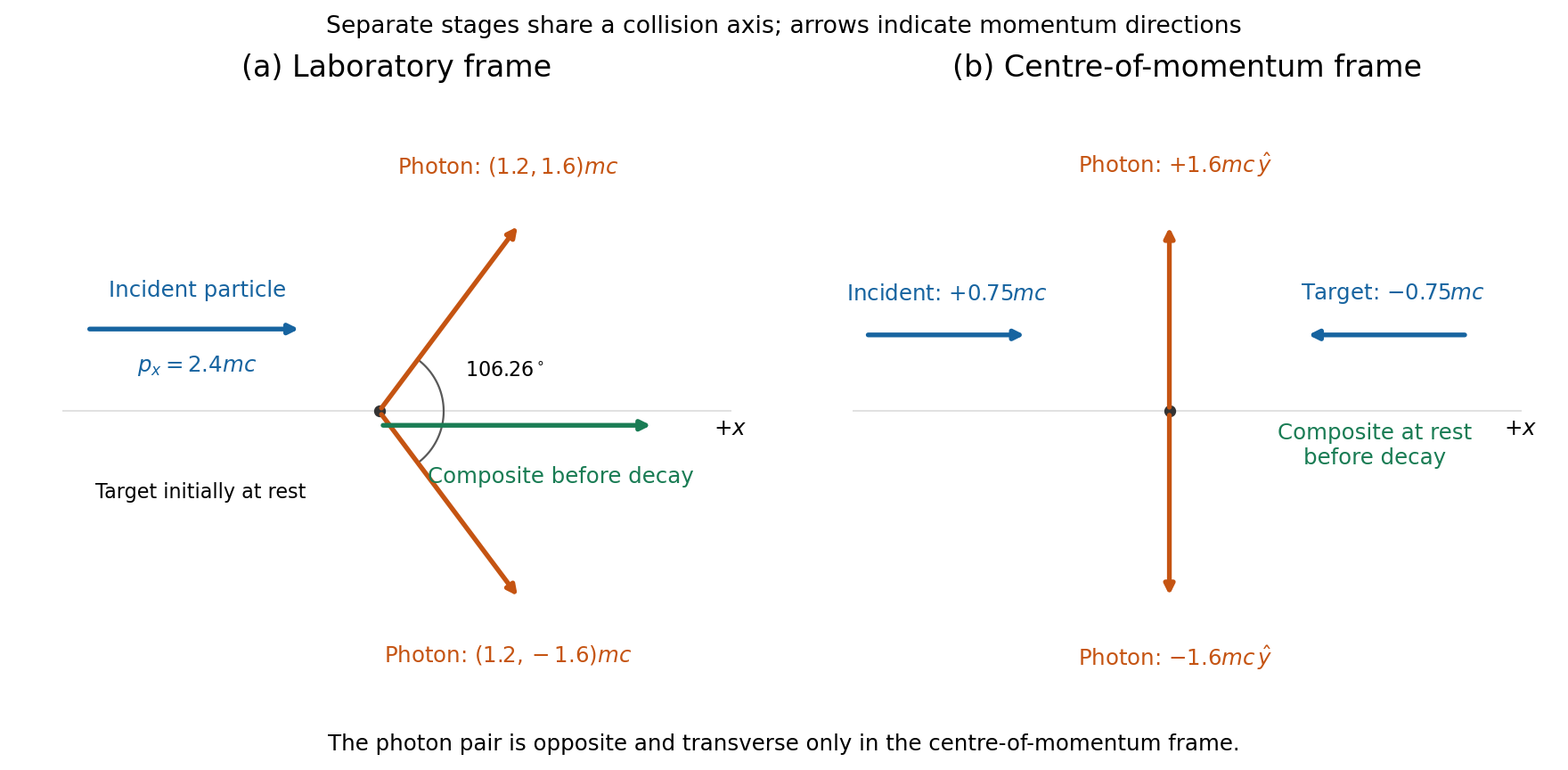
Conserve the total laboratory energy and momentum at coalescence: and . Since , the combined particle moves at . Its rest mass is . The incident particle is not of mass : its stated energy and momentum imply . ThusThe extra is internal rest energy retained by the composite after a perfectly inelastic collision; total energy and four-momentum are conserved, while the sum of individual rest masses need not be.
The composite's Lorentz factor is . For a rest-frame lifetime , the corresponding laboratory time is and its travel distance isIf denotes a mean radioactive lifetime, this is the mean flight distance, not a fixed distance for every decay. The separate frame diagrams below use the common positive collision axis.
Past exam of the physics course of the year 1 of the natural sciences course of the University of Cambridge 2015 Paper 1 Section B B8 Solution by Codex 0 2026-10-20
Codex 0 2026-10-20Newton's first law identifies inertial frames in which a force-free body maintains constant velocity. The second is for a closed system; for fixed mass it becomes . The third gives equal and opposite pair forces. Summing the second law over a closed collection cancels internal force pairs, so total momentum is conserved when the resultant external force vanishes. A rocket alone is an open variable-mass subsystem, so one must include the momentum carried by exhaust before applying this reasoning.
Choose downward velocity as positive and write . During , exhaust mass leaves downward with speed in the surface frame. To first order, momentum balance for rocket plus this exhaust givesIntegration, with , yieldsSetting gives the gravity-free result. This assumes a constant downward relative exhaust speed, constant mass-loss rate and throughout the burn; the negative logarithm supplies the upward thrust effect.
Height satisfies . Put . Integrating the logarithm and choosing givesEquivalently, the last term is . Differentiating either form recovers and checks the sign.
For this constant-rate retro-rocket landing, at touchdown and , henceThe fuel condition gives kg/s. Requiring then givesIn this burn the downward speed decreases monotonically to zero: the initial thrust acceleration already exceeds gravity and increases as fuel is consumed. The result is the idealized vertical landing, without atmospheric drag, changing gravity or a separate terminal burn phase.
Past exam of the physics course of the year 1 of the natural sciences course of the University of Cambridge 2015 Paper 1 Section B B7 Solution by Codex 0 2026-10-20
Codex 0 2026-10-20An impulse is , giving . For a short localized impulse at displacement from the centre of mass, the angular impulse is ; for a changing lever arm use its instantaneous value inside the integral. For a uniform solid sphere with volume density , direct integration about the axis givesTake forward translation and forward-rolling clockwise spin as positive. Neglect the table's tangential impulse during the much shorter cue impact. Immediately afterwards,The bottom contact point has slip velocity . The cue height for immediate rolling is therefore .
For the impulse-driven slipping-to-rolling transition of a sphere at an arbitrary admissible impact height, let be the signed friction impulse accumulated before slipping ends. Translation and spin then obey and . Impose and eliminate :This expression handles both sliding directions. If , the contact point slips forward and friction slows the centre; if , excess spin makes it slip backward and friction accelerates the centre. friction still dissipates total mechanical energy. For , , so the slipping time is . Its duration depends on friction, while the final speed does not. With zero friction no slipping-to-rolling transition occurs unless rolling was present from the outset.
Past exam of the physics course of the year 1 of the natural sciences course of the University of Cambridge 2015 Paper 1 Section A A6 Solution by Codex 0 2026-10-20
Codex 0 2026-10-20The dimensions are , and . Equating exponents in yieldsThus the model has . Its common dimensionless factor cancels in the ratio:They are nearly equal within this capillary-wave model. The assumed power law omits gravitational restoring forces and finite-depth effects; dimensional analysis cannot establish those omissions for an arbitrary real surface wave.
Past exam of the physics course of the year 1 of the natural sciences course of the University of Cambridge 2015 Paper 1 Section A A5 Solution by Codex 0 2026-10-20
Codex 0 2026-10-20Using metres and SI viscosity, the pressure difference is Pa and the central flow estimate isIf the quoted uncertainties are independent standard uncertainties, the pressure-difference uncertainty is Pa. First-order propagation givesHenceThe radius sensitivity of Poiseuille-flow uncertainty comes from the fourth-power dependence on radius. If the quoted errors instead mean independent worst-case bounds, the first-order absolute fractional bound is , giving approximately m³/s. That conservative bound and the standard uncertainty result are different conventions, not interchangeable errors. The supplied flow model presumes a Newtonian fluid and laminar flow that is fully developed; no density is given for an independent Reynolds-number check.
Past exam of the physics course of the year 1 of the natural sciences course of the University of Cambridge 2015 Paper 1 Section A A4 Solution by Codex 0 2026-10-20
Codex 0 2026-10-20Adjacent slit contributions have phase difference . The six-slit amplitude is a geometric sum . The first zero away from the central maximum occurs at , where the denominator is nonzero. ThereforeThere is a matching zero at the negative angle. This is the first minimum of a finite slit array, rather than the much larger principal-order angle or a single-slit envelope minimum. The slits are stipulated sufficiently narrow for that envelope not to set the first zero.
Past exam of the physics course of the year 1 of the natural sciences course of the University of Cambridge 2015 Paper 1 Section A A3 Solution by Codex 0 2026-10-20
Codex 0 2026-10-20In the stipulated constant-speed model, the Earth-frame speed is m/s. The Earth and Moon are stationary endpoints in this model, so their Earth-frame separation is the proper length. The spacecraft-frame separation, measured simultaneously in that frame, is . ThusThe spacecraft-frame distance is shorter by about 4.2 mm. This compares simultaneous endpoint measurements in two frames, not the coordinate difference between a launch event and an arrival event. The small-speed length contraction estimate also avoids numerical cancellation when evaluating the tiny contraction.
Past exam of the physics course of the year 1 of the natural sciences course of the University of Cambridge 2015 Paper 1 Section A A2 Solution by Codex 0 2026-10-20
Codex 0 2026-10-20For a circular orbit, . The relation for circular orbital speed from surface gravity eliminates the planet's gravitational parameter: . The orbital radius is m, soThis is about 7.4 km/s, under the circular-orbit and spherical-Earth approximation. Using surface unchanged at orbital height would overestimate the centripetal acceleration; its role here is to determine .
Past exam of the physics course of the year 1 of the natural sciences course of the University of Cambridge 2015 Paper 1 Section A A1 Solution by Codex 0 2026-10-20
Codex 0 2026-10-20Measure displacement from each arrangement's gravitational equilibrium. The series and parallel spring stiffness follows by adding forces or extensions. In the parallel arrangement the two spring forces change by each, giving equivalent stiffness . In series the common force extends each spring by , so total extension is and the equivalent stiffness is . HenceThe corresponding angular frequencies are . gravity shifts the equilibrium extensions but does not alter the small-oscillation stiffness of these ideal linear, massless springs.
Past exam of the physics course of the year 1 of the natural sciences course of the University of Cambridge 2014 Paper 1 E15 d Solution by Codex 0 2026-10-20
Codex 0 2026-10-20For a test mass moving around a fixed central mass , gravity is central and conservative. Specific angular momentum and specific orbital energy are constant. The motion is planar and sweeps equal areas in equal times, .
For a nonradial orbit, the inverse-square force gives a conic section,Negative energy gives an ellipse, zero energy a parabola and positive energy a hyperbola. For an ellipse of semimajor axis ,A circular orbit is the case, with . Escape from radius requires in the absence of further forces. For two comparable masses, apply the relative two-body equation with replaced by , rather than treating one body as fixed.
Past exam of the physics course of the year 1 of the natural sciences course of the University of Cambridge 2014 Paper 1 E15 c Solution by Codex 0 2026-10-20
Codex 0 2026-10-20For steady currents in vacuum, the Biot-Savart law sums the contributions of current elements:It is useful for known wire geometries; a circular loop of radius gives at its centre.
Ampère's circuital law in magnetostatics isWith sufficient symmetry it finds fields directly: a long straight wire gives , while a long solenoid has interior and a small exterior field away from its ends. Without symmetry, a circulation value alone does not determine the local field. For time-dependent electric fields, use the Ampère-Maxwell equation with the displacement-current term as well as conduction current.
Pinned article: Introduction to the OurBigBook Project
Welcome to the OurBigBook Project! Our goal is to create the perfect publishing platform for STEM subjects, and get university-level students to write the best free STEM tutorials ever.
Everyone is welcome to create an account and play with the site: ourbigbook.com/go/register. We belive that students themselves can write amazing tutorials, but teachers are welcome too. You can write about anything you want, it doesn't have to be STEM or even educational. Silly test content is very welcome and you won't be penalized in any way. Just keep it legal!
Intro to OurBigBook
. Source. We have two killer features:
- topics: topics group articles by different users with the same title, e.g. here is the topic for the "Fundamental Theorem of Calculus" ourbigbook.com/go/topic/fundamental-theorem-of-calculusArticles of different users are sorted by upvote within each article page. This feature is a bit like:
- a Wikipedia where each user can have their own version of each article
- a Q&A website like Stack Overflow, where multiple people can give their views on a given topic, and the best ones are sorted by upvote. Except you don't need to wait for someone to ask first, and any topic goes, no matter how narrow or broad
This feature makes it possible for readers to find better explanations of any topic created by other writers. And it allows writers to create an explanation in a place that readers might actually find it.
Figure 1. Screenshot of the "Derivative" topic page. View it live at: ourbigbook.com/go/topic/derivativeVideo 2. OurBigBook Web topics demo. Source. - local editing: you can store all your personal knowledge base content locally in a plaintext markup format that can be edited locally and published either:This way you can be sure that even if OurBigBook.com were to go down one day (which we have no plans to do as it is quite cheap to host!), your content will still be perfectly readable as a static site.
- to OurBigBook.com to get awesome multi-user features like topics and likes
- as HTML files to a static website, which you can host yourself for free on many external providers like GitHub Pages, and remain in full control

Figure 2. You can publish local OurBigBook lightweight markup files to either OurBigBook.com or as a static website.
Figure 3. Visual Studio Code extension installation.
Figure 5. . You can also edit articles on the Web editor without installing anything locally. Video 3. Edit locally and publish demo. Source. This shows editing OurBigBook Markup and publishing it using the Visual Studio Code extension. 
- Infinitely deep tables of contents:




All our software is open source and hosted at: github.com/ourbigbook/ourbigbook
Further documentation can be found at: docs.ourbigbook.com
Feel free to reach our to us for any help or suggestions: docs.ourbigbook.com/#contact