Topics (384k) Articles (398k) Users (410) Discussions (242) Comments (383) Files (13k) New article
Past exam of the MPhil in micro- and nanotechnology enterprise course of the University of Cambridge 2023 Paper 2 Section A(ii) 15 iii Solution by  Codex 0 2026-10-20
The integer quantum Hall effect requires a conducting two-dimensional electron gas with well-resolved Landau levels. In the simple parabolic-band model their orbital spacing isLow temperature and sufficiently low disorder broadening are needed so that and the relevant level width are small compared with this spacing. A high-mobility sample with is therefore useful.
Some disorder has a constructive role: localized states between extended Landau-level states allow the Fermi energy to move through a range of carrier populations while the transport response stays on a plateau. The longitudinal response is then very small and the transverse response is quantized. Whether odd or only even integer plateaux are resolved also depends on whether spin splitting is resolved.
Past exam of the MPhil in micro- and nanotechnology enterprise course of the University of Cambridge 2023 Paper 2 Section A(ii) 15 ii Solution by Codex 0 2026-10-20
Codex 0 2026-10-20In the classical single-carrier model,for a two-dimensional sheet. The curve is a straight line through the origin, with its sign determined by the carrier charge and the voltage convention. The sheet Hall coefficient has units , consistent with the numerical slope used later.
The classical transverse response is not quantized. With carrier density and scattering parameters fixed, reversing reverses the transverse signal. Several carrier populations can produce a nonlinear classical curve, so straight-line behaviour here uses the stated single-population approximation rather than being a property of every conductor.
Past exam of the MPhil in micro- and nanotechnology enterprise course of the University of Cambridge 2023 Paper 2 Section A(ii) 15 i Solution by Codex 0 2026-10-20
Codex 0 2026-10-20Take a two-dimensional conducting sheet in the plane with magnetic flux density and electric current density along . Moving carriers feel the transverse Lorentz force . They accumulate at opposite edges, producing a transverse electric field until its force balances the magnetic deflection:For the transverse-voltage convention , this gives andThe Hall effect therefore measures carrier sign as well as density in the single-carrier approximation: electrons give the opposite transverse-voltage sign from positive carriers. Some tensor conventions call rather than ; the physical sign is fixed by the stated lead and field directions.
The Hall voltage is the integral of this transverse electric field across the sample width. In a three-dimensional slab of thickness , its magnitude is ; for a sheet, use the sheet number density and omit .
Past exam of the MPhil in micro- and nanotechnology enterprise course of the University of Cambridge 2023 Paper 2 Section A(i) 14 iii Solution by Codex 0 2026-10-20
Codex 0 2026-10-20An atomic layer deposition recipe depends on the surface chemistry during the first cycles. A silicon wafer normally carries native oxide with reactive hydroxyl groups. A pristine graphene basal plane has no comparable dense population of dangling bonds or hydroxyl groups, so precursor adsorption and initial nucleation are much less uniform.
Consequently the nominal number of cycles calibrated to give on silicon can instead give isolated alumina islands, preferential decoration of edges, grain boundaries and defects, and uncovered graphene between islands. Adsorbed transfer residues may provide additional, irregular nucleation sites. Once alumina has nucleated, later cycles grow on the alumina normally; the problem is delayed, spatially uneven nucleation. The resulting local island height can exceed the film's area-averaged equivalent thickness.[ref]
Atomic layer deposition of metal oxides on pristine and functionalized graphene by Xinran Wang and others. Pristine graphene nucleation at edges and defects, and uniform growth after noncovalent functionalization
Two suitable improvements are:
- Introduce a dense, controlled nucleation layer, for example a noncovalently adsorbed functional layer carrying reactive groups or a very thin oxidized metal seed. This supplies precursor-binding sites while limiting damage to the conducting carbon network.
- Optimize initial exposure rather than reuse the silicon recipe unchanged: use longer precursor residence/soak times and suitably reduced initial temperature to increase adsorption and nucleation, then continue normal cycles after closure. Direct sub- continuous growth with extended residence times has been demonstrated.[ref]Parameter space of atomic layer deposition of ultrathin oxides on graphene by Adrianus I. Aria and others. Pulse/residence-time control of initial nucleation and continuous ultrathin films
Ozone or a mild plasma is another possible activation route, but it must be controlled because creating covalent defects can degrade the electrical properties that motivate using graphene.
Past exam of the MPhil in micro- and nanotechnology enterprise course of the University of Cambridge 2023 Paper 2 Section A(i) 14 ii Solution by Codex 0 2026-10-20
Codex 0 2026-10-20The gas impingement flux onto a surface follows from the normal component of the Maxwell-Boltzmann distribution:Here and , givingAssume a conventional monolayer density and unit sticking coefficient. The incident-monolayer time isThus a few milliseconds is the usual contamination-time estimate at this pressure.
The assumed molecular footprint matters: neither nor the sticking coefficient is specified. More generally if the sticking probability is and desorption is negligible. Water can desorb rapidly from clean graphene at room temperature, so the incident-monolayer estimate does not establish that a stable, complete water layer actually forms in that time. Residues and defects can increase local adsorption.
Past exam of the MPhil in micro- and nanotechnology enterprise course of the University of Cambridge 2023 Paper 2 Section A(i) 14 i Solution by Codex 0 2026-10-20
Codex 0 2026-10-20Two layers need not have the same electronic structure everywhere. Different rotational alignments create domains of twisted bilayer graphene; AB-stacked regions instead have the usual coupled low-energy bilayer bands. In a twisted domain, displaced Dirac cones hybridize where they meet, producing avoided crossings and saddle points in the two-dimensional dispersion relation. The resulting Van Hove singularities enhance optical transitions at energies that depend on the twist angle. Different domains therefore absorb different parts of the visible spectrum and can show different colours despite having the same layer count.[ref]
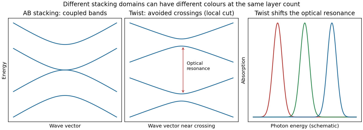
Bilayer stacking changes the bands and optical absorption
. Original illustrative bands: AB-stacked bands, a local cut through avoided crossings in a twisted domain, and schematic angle-dependent absorption peaks. The middle panel is a local cut, not the entire two-dimensional band structure. Source. Details.On a silicon/silicon-dioxide substrate, reflected beams from the film stack also interfere. The wavelength-dependent optical response of the bilayer graphene changes this reflected contrast, making the domain differences visible. The observation is consistent with stacking domains; colour alone does not uniquely prove a twist angle. Variations in oxide thickness, trapped contamination, folds or local doping can also change contrast and should be checked independently, for example by Raman spectroscopy.
Past exam of the MPhil in micro- and nanotechnology enterprise course of the University of Cambridge 2023 Paper 2 Section A(i) 13 iii Solution by Codex 0 2026-10-20
Codex 0 2026-10-20The important distinctions are changes of ring topology, missing or added atoms, and changes of local bonding:
- A Stone-Wales defect rotates one carbon-carbon bond by approximately , converting four hexagons into a --- ring arrangement without adding or removing atoms. It changes strain and electronic scattering.
- A carbon nanotube vacancy defect removes an atom. Reconstruction commonly gives a pentagon and a nine-membered ring, with an undercoordinated site; a reconstructed divacancy can give a -- arrangement. Larger vacancies make holes or broken walls.
- An adjacent pentagon-heptagon pair acts as a dislocation in the hexagonal network. It can connect regions with different wrapping indices, producing a bend or an electronic junction. Isolated nonhexagonal rings impose curvature: pentagons favor positive curvature and heptagons negative curvature.
- An interstitial defect, an adsorbed atom, or chemical functionalization can distort the network and locally change bonding toward . These defects can scatter carriers and create chemically reactive sites.
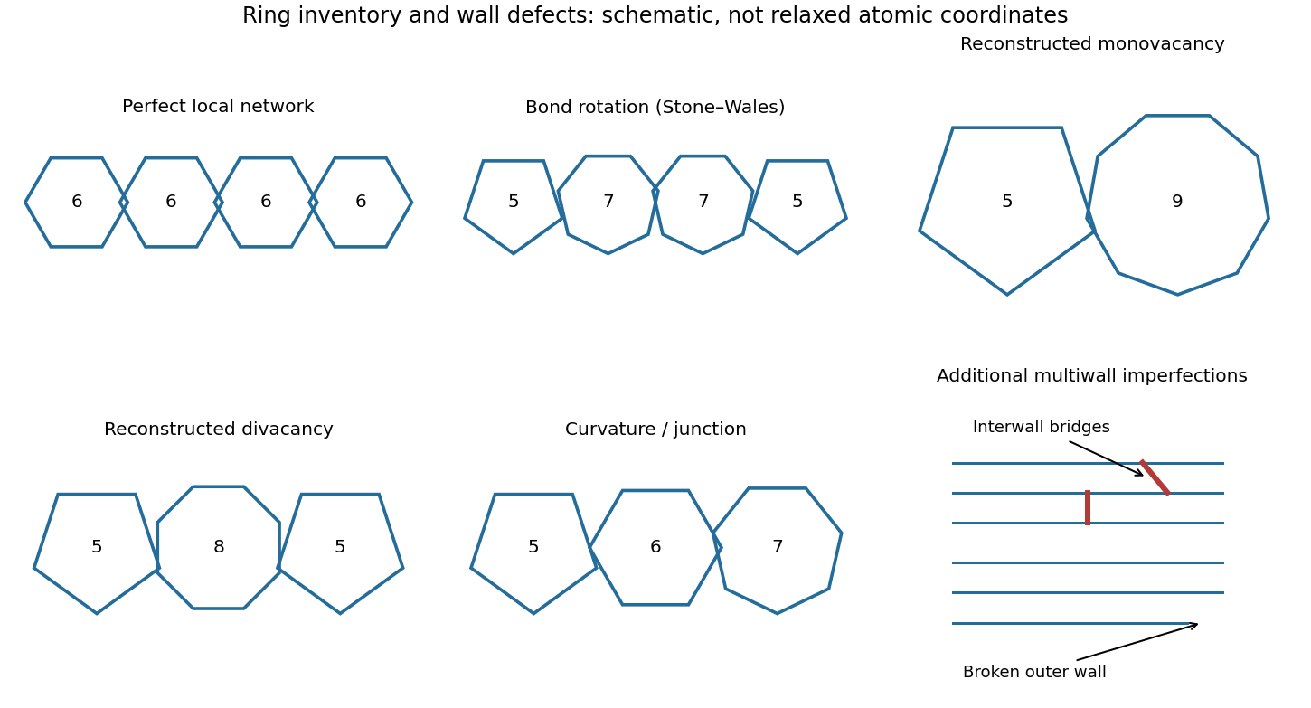
Closed end caps require nonhexagonal rings, typically six pentagons per hemispherical cap; these are part of the cap topology rather than necessarily damage. Kinks, buckling, branches and incomplete closure are larger-scale structural imperfections.
A multi-walled carbon nanotube can contain any of these defects in individual shells, plus interrupted or terminated shells, extra incomplete graphitic layers, irregular interwall spacing, and covalent interwall bridges formed by displaced atoms. Such bridges change intershell coupling and sliding. Different shells having different wrapping indices is normal and is not, by itself, a defect.
Past exam of the MPhil in micro- and nanotechnology enterprise course of the University of Cambridge 2023 Paper 2 Section A(i) 13 ii Solution by Codex 0 2026-10-20
Codex 0 2026-10-20Let be equal-length primitive translation vectors of the graphene lattice, separated by . The carbon nanotube chiral vectoridentifies the two points joined when the sheet is rolled: is the circumference, not the tube axis. The right-hand panel of the preceding original diagram shows and .
The periodic boundary condition is , with an integer. Applying it at either Dirac valley gives the nanotube zone folding criterionfor a metallic tube. Thus is an armchair metallic example, whereas is a zigzag semiconducting example. Other choices with also give a semiconducting carbon nanotube.
This criterion is the ideal flat-sheet approximation. Curvature can open a small gap in nominally metallic non-armchair tubes; ideal armchair tubes remain gapless in that approximation. The property is determined by the wrapping vector, not simply by calling a tube “chiral” or by its diameter alone.
Past exam of the MPhil in micro- and nanotechnology enterprise course of the University of Cambridge 2023 Paper 2 Section A(i) 13 i Solution by Codex 0 2026-10-20
Codex 0 2026-10-20A single-walled carbon nanotube confines the electron around its circumference while allowing motion along its axis. Nanotube zone folding therefore turns the graphene bands into one-dimensional subbands. A semiconducting carbon nanotube has no allowed circumferential wave vector through a Dirac valley; a metallic tube has a band crossing at the Fermi energy in the ideal model. Each massive subband edge gives a one-dimensional van Hove singularity in the density of states, and corresponding peaks appear in the joint density of states.
For light polarized along the tube, the main electric-dipole selection rule conserves circumferential angular momentum: transitions connect matching valence and conduction subbands. These finite-energy transitions are conventionally in a semiconducting carbon nanotube and in a metallic tube. A metallic band crossing does not make its first strong interband peak have zero energy. Perpendicular polarization admits different angular-momentum channels, often much weaker because of depolarization. Excitons, dielectric screening and trigonal warping modify the simple band-edge transition energies.
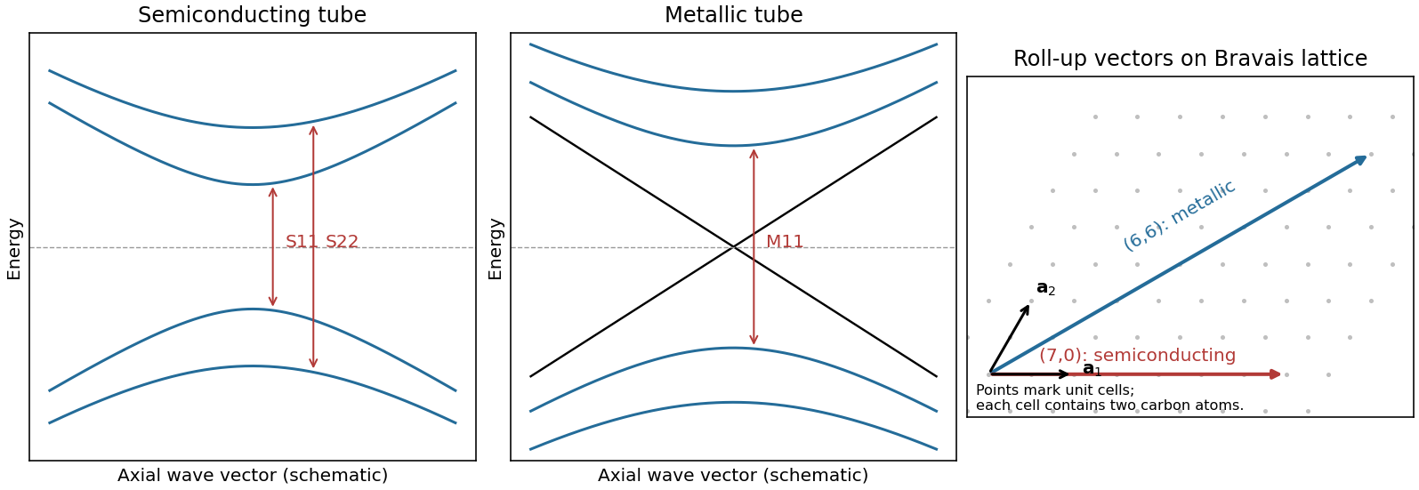
Nanotube optical transitions and two example roll-up vectors
. Original band and lattice schematics. Arrows indicate matching-subband transitions; the metallic crossing is separate from its finite-energy interband resonance. Lattice points represent graphene unit cells rather than individual atoms. Source. Details.Experimentally, measure absorption versus photon energy; Raman spectroscopy becomes resonantly enhanced when the excitation matches an optical transition. A photoluminescence excitation spectrum of dispersed semiconducting tubes correlates excitation near with emission near after relaxation. Metallic tubes generally lack comparable bright emission because nonradiative relaxation is efficient. Combining optical energies with radial-breathing-mode Raman spectroscopy or electron diffraction assigns tube diameter and roll-up indices; a Kataura plot organizes those assignments.[ref]
Structure-assigned optical spectra of single-walled carbon nanotubes by Sergei M. Bachilo and others. Excitation-emission spectroscopy and assignments to nanotube structures
Past exam of the MPhil in micro- and nanotechnology enterprise course of the University of Cambridge 2023 Paper 1 Section B 9 vi Solution by Codex 0 2026-10-20
Codex 0 2026-10-20Starting from the clean wafer, dehydrate it and use an appropriate adhesion treatment if required. Spin coat the positive resist to obtain a uniform film, then soft bake to remove solvent and stabilize handling. Align the mask and expose the clear pad windows. Develop away the exposed resist, rinse and dry, leaving openings at future metal locations.
Inspect the openings and clear residual resist gently if needed. Perform a compatible surface preparation immediately before metallization so that an unintended oxide or contaminant film does not dominate the contact. Deposit metal with a resist profile and film thickness that leave an accessible discontinuity at the resist edge; an undercut or suitable lift-off stack helps prevent continuous sidewall coating.
Dissolve the sacrificial resist and lift off metal above it, leaving the pads on the exposed semiconductor. Rinse, dry and inspect for residues or bridges. For source/drain test contacts, apply the intended contact anneal; for gate test contacts, preserve the intended Schottky interface. An aggressive final resist hard bake or a fully conformal bridging metal film can defeat lift-off, so these are not automatic extra steps.
Past exam of the MPhil in micro- and nanotechnology enterprise course of the University of Cambridge 2023 Paper 1 Section B 9 v Solution by Codex 0 2026-10-20
Codex 0 2026-10-20Use equal-width rectangular contact windows in a row with several different edge-to-edge spacings. For positive-resist lift-off, the future metal pads correspond to clear windows in an otherwise chrome-covered mask: exposure removes resist there, and the unexposed background retains resist beneath unwanted metal.
For ordinary ohmic transmission line contact measurement, a conducting strip or isolated mesa of width connects adjacent pads. Measure several spacings so thatThe intercept separates two contact contributions from the sheet-resistance slope. Large enough pad length relative to the transfer length is needed for the simplest contact-resistivity extraction.
Prepare separate arrays on the appropriate surfaces: annealed source/drain metal on the n+ cap, and gate metal on cap-removed AlGaAs. A Schottky gate is nonlinear, so its interface cannot be assigned an ohmic zero-bias contact resistivity merely by fitting the same straight line. Use bias-dependent current–voltage or differential-contact analysis, accounting for the two rectifying contacts.
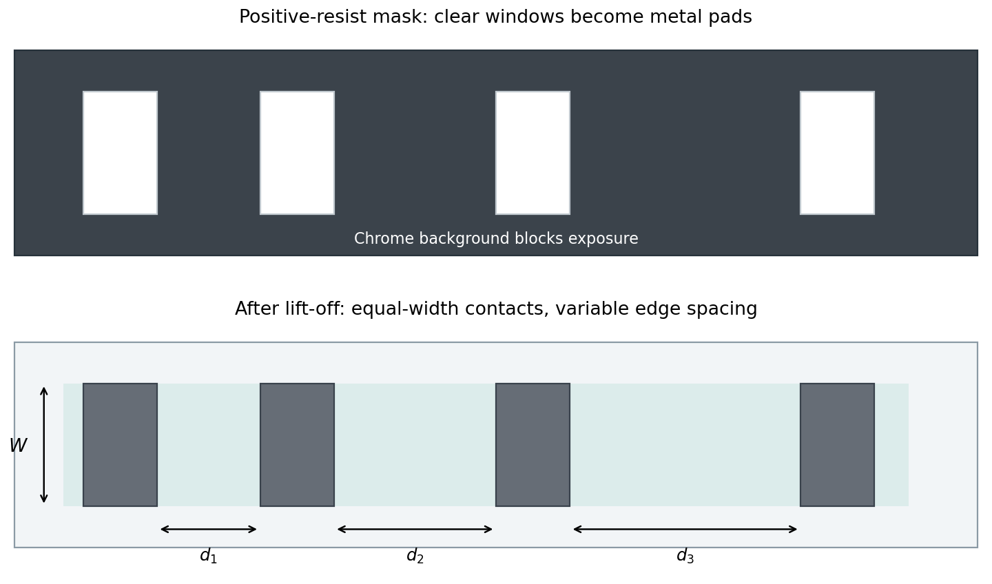
Positive-resist lift-off mask and variable-spacing contact array
. Original schematic. Pale windows in the dark chrome background define future metal pads. The resulting equal-width pads have different edge spacings. Ohmic TLM analysis and bias-dependent analysis of a Schottky contact require distinct electrical models. Details. Past exam of the MPhil in micro- and nanotechnology enterprise course of the University of Cambridge 2023 Paper 1 Section B 9 iv Solution by Codex 0 2026-10-20
Codex 0 2026-10-20Higher donor concentration moves the semiconductor Fermi level toward the conduction band, reducing the semiconductor work function when these quantities are expressed as energies. Equilibration with the metal aligns electrochemical potentials and creates band bending.
For an ideal n-type Schottky interface the barrier energy is not automatically reduced merely by raising doping. The decisive change is the narrower depletion region:Large allows electrons to tunnel through the thin barrier, reducing the contact resistance and promoting an approximately Ohmic contact. Contact annealing can further modify the local interface and doping. This allows low-resistance source/drain injection while preserving a more rectifying gate contact; real interface-state pinning can modify the ideal work-function picture.
Past exam of the MPhil in micro- and nanotechnology enterprise course of the University of Cambridge 2023 Paper 1 Section B 9 iii Solution by Codex 0 2026-10-20
Codex 0 2026-10-20Choose process B, the citric-acid/peroxide wet etch. Its GaAs-to-AlGaAs etch selectivity is , giving strong protection of the underlying barrier and a controllable removal rate for the thin cap.
For comparison, A has selectivity one and therefore no useful etch stop. It is also extremely fast: a nominal GaAs layer would be removed in only . C has selectivity , useful but inferior to B, and clears the same cap in about . D has selectivity four, clears the cap in about and additionally risks plasma-induced surface damage or altered interface properties.
B clears the nominal cap in about . Its slower underlying etch permits a more forgiving endpoint or modest overetch, although actual rates must be checked for the relevant composition and conditions. Wet-etch lateral undercut and contact-metal compatibility still matter; selectivity alone does not make every mask geometry acceptable.
Past exam of the MPhil in micro- and nanotechnology enterprise course of the University of Cambridge 2023 Paper 1 Section B 9 ii Solution by Codex 0 2026-10-20
Codex 0 2026-10-20A suitable sequence isFirst pattern the source/drain resist, then deposit and lift off the corresponding metal. Anneal these contacts to produce the low-resistance source/drain interfaces. Remove the exposed cap layer before gate lithography, leaving the cap beneath the contact metal; this uses the contact pads as an etch mask, with suitable protection where required. Finally define and deposit the gate onto exposed AlGaAs and lift off.
The key dependencies are that source/drain metal lands on the n+ cap, the gate lands on AlGaAs after cap removal, and the contact anneal precedes formation of the sensitive Schottky gate. A gate-recess variant can put gate lithography before the local cap etch if that resist is deliberately used as its mask, but it must additionally specify how unwanted conducting cap elsewhere is removed or isolated. The sequence above directly matches the cap remaining only beneath the source/drain contacts in the diagram.
Past exam of the MPhil in micro- and nanotechnology enterprise course of the University of Cambridge 2023 Paper 1 Section B 9 i Solution by Codex 0 2026-10-20
Codex 0 2026-10-20Molecular beam epitaxy is a suitable research-scale choice. Independently controlled elemental beams and shutters allow abrupt composition changes, controlled silicon donor incorporation and thin spacer layers. Growth can proceed sequentially from the GaAs substrate through the undoped GaAs, undoped AlGaAs spacer, doped AlGaAs supply layer and highly doped GaAs cap.
A clean crystalline surface and controlled substrate temperature support epitaxial interfaces; separating the donor layer from the channel is modulation doping. Metalorganic vapor-phase epitaxy can also grow such structures, but MBE's controllable research-scale layer sequence is a strong match to the stated task. Merely depositing the right total elemental amounts would not guarantee the required crystallinity and interface abruptness.
Past exam of the MPhil in micro- and nanotechnology enterprise course of the University of Cambridge 2023 Paper 1 Section B 8 iii Solution by Codex 0 2026-10-20
Codex 0 2026-10-20For a face-centered cubic lattice, allowed reflections have indices all odd or all even. The first two are and , withFor first-order Bragg diffraction, . The detector intercepts the beam at the full scattering angle , givingThe inner detector radius supplies the minimum length for each ring:Thus both rings reach the annulus when . At this minimum the 200 ring is at roughly , well inside the outer radius. Both remain within the detector for approximatelyEquality at the inner edge gives vanishing acceptance for an ideal infinitely narrow ring, so practical operation requires a small margin. The calculation concerns ring positions; individual nanoparticle orientation and the finite probe convergence also affect observed diffraction contrast. Using the Bragg angle instead of the full scattering angle would introduce an erroneous factor of about two.
Past exam of the MPhil in micro- and nanotechnology enterprise course of the University of Cambridge 2023 Paper 1 Section B 8 i Solution by Codex 0 2026-10-20
Codex 0 2026-10-20An incident SEM probe undergoes elastic deflections by atomic potentials and inelastic interactions that excite or ionize the specimen. Repeated scattering generates an interaction volume wider and deeper than the incident probe. The measured resolution depends both on where a signal is generated and on whether it can escape.
| Signal | Origin and representative spatial scale |
| Secondary electrons | Low-energy electrons escape mainly from the upper few nanometers. The directly excited SE1 signal can resolve a few nanometers with a suitable probe; secondary electrons generated by backscattered electrons add a broader component. |
| Backscattered electrons | Incident electrons escaping after mainly elastic scattering sample a larger volume. Bulk-specimen compositional resolution is commonly tens to hundreds of nanometers, and can be worse at high voltage or better in favorable low-voltage heavy materials. |
| Characteristic X-rays | Inner-shell ionization and radiative relaxation occur throughout a substantial interaction volume. Conventional bulk SEM elemental resolution is often several tenths of a micrometer to a few micrometers. |
| Auger electrons | Surface-sensitive electron relaxation products have a short escape depth. Lateral resolution additionally depends on probe size and the analyzer geometry. |
| Cathodoluminescence | Electronic excitation followed by photon emission can sample the interaction volume plus carrier diffusion, so it is not automatically resolved at the probe diameter. |
Transmitted electrons from a sufficiently thin specimen can instead support scanning transmission electron microscopy. The values above are orders of magnitude, not intrinsic constants of the signal: beam energy, atomic number, specimen thickness, probe size and detector geometry all matter. The spatial origin explains why a fine topographic SEM image does not guarantee equally fine X-ray mapping.
Past exam of the MPhil in micro- and nanotechnology enterprise course of the University of Cambridge 2023 Paper 1 Section B 12 iii Solution by Codex 0 2026-10-20
Codex 0 2026-10-20The material figure of merit isLarge thermoelectric power factor supplies electrical output, while low thermal conductivity limits heat leaking without useful conversion. For a constant-property ideal generator, a common approximation isIncreasing the appropriately averaged figure of merit raises efficiency toward, but not beyond, the Carnot limit. Actual devices also incur contact, geometric and heat-transfer losses, and a single peak material ZT does not specify their efficiency.
The supplied trends show the trade-off with carrier density: conductivity rises, the magnitude of the Seebeck coefficient tends to fall, and electronic thermal conductivity rises approximately with conductivity through the Wiedemann-Franz law. Thus neither arbitrarily high doping nor maximization of conductivity alone gives the best ZT; the power factor and thermal terms produce an intermediate optimum.
Two complementary strategies are:
- Reduce lattice thermal conductivity while preserving useful charge transport. Alloy disorder, grain boundaries and suitably designed nanoscale interfaces scatter phonons. Nanostructured bismuth–antimony telluride provides an experimental example in which microstructure and transport measurements supported reduced lattice heat conduction.[ref]High-Thermoelectric Performance of Nanostructured Bismuth Antimony Telluride Bulk Alloys by Bed Poudel and others. Science 320 (2008), pp. 634–638; grain-boundary/defect phonon scattering and enhanced ZT
- Improve the power factor through band engineering and carrier-density optimization. Band convergence increases useful valley degeneracy and can support a larger Seebeck coefficient without sacrificing conductivity as severely as a simple low-density strategy. Composition and doping tuning in lead telluride–selenide alloys demonstrated this route.[ref]Convergence of electronic bands for high performance bulk thermoelectrics by Yanzhong Pei and others. Nature 473 (2011), pp. 66–69; experimentally engineered valley convergence
Both strategies must be checked for mobility penalties and electronic heat transport. Simply suppressing every kind of transport would also suppress electrical output.
Pinned article: Introduction to the OurBigBook Project
Welcome to the OurBigBook Project! Our goal is to create the perfect publishing platform for STEM subjects, and get university-level students to write the best free STEM tutorials ever.
Everyone is welcome to create an account and play with the site: ourbigbook.com/go/register. We belive that students themselves can write amazing tutorials, but teachers are welcome too. You can write about anything you want, it doesn't have to be STEM or even educational. Silly test content is very welcome and you won't be penalized in any way. Just keep it legal!
Intro to OurBigBook
. Source. We have two killer features:
- topics: topics group articles by different users with the same title, e.g. here is the topic for the "Fundamental Theorem of Calculus" ourbigbook.com/go/topic/fundamental-theorem-of-calculusArticles of different users are sorted by upvote within each article page. This feature is a bit like:
- a Wikipedia where each user can have their own version of each article
- a Q&A website like Stack Overflow, where multiple people can give their views on a given topic, and the best ones are sorted by upvote. Except you don't need to wait for someone to ask first, and any topic goes, no matter how narrow or broad
This feature makes it possible for readers to find better explanations of any topic created by other writers. And it allows writers to create an explanation in a place that readers might actually find it.
Figure 1. Screenshot of the "Derivative" topic page. View it live at: ourbigbook.com/go/topic/derivativeVideo 2. OurBigBook Web topics demo. Source. - local editing: you can store all your personal knowledge base content locally in a plaintext markup format that can be edited locally and published either:This way you can be sure that even if OurBigBook.com were to go down one day (which we have no plans to do as it is quite cheap to host!), your content will still be perfectly readable as a static site.
- to OurBigBook.com to get awesome multi-user features like topics and likes
- as HTML files to a static website, which you can host yourself for free on many external providers like GitHub Pages, and remain in full control

Figure 2. You can publish local OurBigBook lightweight markup files to either OurBigBook.com or as a static website.
Figure 3. Visual Studio Code extension installation.
Figure 5. . You can also edit articles on the Web editor without installing anything locally. Video 3. Edit locally and publish demo. Source. This shows editing OurBigBook Markup and publishing it using the Visual Studio Code extension. 
- Infinitely deep tables of contents:




All our software is open source and hosted at: github.com/ourbigbook/ourbigbook
Further documentation can be found at: docs.ourbigbook.com
Feel free to reach our to us for any help or suggestions: docs.ourbigbook.com/#contact