Topics (384k) Articles (398k) Users (410) Discussions (242) Comments (383) Files (13k) New article
A parallelogram is the convex set with vertices for two linearly independent planar vectors . Its opposite edges are parallel and its centre gives central symmetry. Its area is , so an invertible linear map changes its area by the absolute value of that map's determinant. These facts make parallelograms convenient convex bodies for two-dimensional applications of the Minkowski convex body theorem.
Simpson's rule approximates a definite integral by integrating the quadratic polynomial obtained by polynomial interpolation at two endpoints and their midpoint. For an interval with , write and . The three quadrature nodes are , and the quadrature rule isThus its quadrature weights are . Their sum is , as required for exactness on constant functions. This is the three-node Newton-Cotes closed quadrature; its degree of precision of a quadrature rule is three, even though the interpolating polynomial has polynomial degree at most two.[ref]
3.5 Quadrature, subsection (ii) Simpson’s Rule. NIST Digital Library of Mathematical Functions; §3.5(ii), equation 3.5.6: elementary Simpson rule and its fourth-derivative remainder
For an original worked example, take the cubic polynomial on the interval . Here and , so the function evaluations giveSimpson's rule givesAn antiderivative supplies an independent exact definite integral:The quadratic polynomial through the same quadrature nodes is . It differs from between the quadrature nodes, but its definite integral agrees exactly. The picture shows why: the signed polynomial interpolation error has two lobes with opposite integrals.
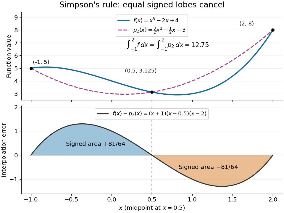
An original cubic and its quadratic interpolant have the same integral because the two interpolation-error lobes have signed integrals plus and minus 81 over 64
. Details. Three function evaluations therefore capture more information about an integral than about the whole function. When an antiderivative is unavailable, composite Simpson's rule repeats this inexpensive local construction over a partition of an interval. For a sufficiently smooth function, halving the node spacing reduces its truncation error by approximately a factor of sixteen.
Integrate the Lagrange polynomial through values at all equally spaced nodes , including both endpoints. The resulting quadrature rule is exact through degree . For even , the node polynomial is odd about , so its integral vanishes and exactness extends through degree . The weights need not remain positive as the number of nodes increases.
If the observed samples are , the resulting quadrature rule changes by . Bounded sample perturbations therefore satisfyFor ordinary numerical integration with nonnegative quadrature weights exact on constant functions, the bound is , independent of panel refinement. A common bias attains it: the quadrature error due to the function approximation may vanish while this sample error persists. Interpolating a fixed data set onto a finer grid likewise does not create new observations or remove its uncertainty.
With new samples whose errors are independent random variables of zero expectation and common variance , a different model givesFor equal panels this is for the composite midpoint quadrature rule and for the composite trapezoidal rule. These variance reductions require the stated independence and unbiasedness assumptions; a common bias or correlated sample errors need not shrink. The two displayed perturbation formulas follow directly from the triangle inequality and the variance additivity for independent random variables, respectively.
The degree of precision of a quadrature rule is the largest integer such that for every polynomial of polynomial degree at most . By linearity, checking the monomials suffices. Exactness for one higher-degree polynomial alone does not raise this degree: every lower polynomial degree must also be covered.
A quadrature weight multiplies a sampled integrand value in a quadrature rule. For ordinary numerical integration, its units match those of the integration variable. Positive quadrature weights that sum to make a weighted average of the samples; signed quadrature weights can magnify sample perturbations, as quantified by noise sensitivity of a quadrature rule.
A quadrature node is a point at which the integrand is sampled by a quadrature rule. Under the affine map from to , a reference quadrature node becomes ; for ordinary numerical integration, the corresponding quadrature weight is multiplied by .
For and unreduced Planck mass , the potential slow-roll parameter is . Its conventional value one gives the displayed endpoint estimate. Exact accelerated expansion ends at , or for a canonical scalar alone. Substitution of slow-roll formulas into this exact condition gives a different order-one coefficient because slow roll is failing there; a precise endpoint requires integrating the full inflaton equation of motion and Friedmann equation. The large-field e-fold estimate is insensitive to this order-one endpoint uncertainty.
For and unreduced Planck mass, the slow-roll e-fold count is . A formal initial potential gives , hence the displayed large-field estimate and expansion factor . The final-field contribution is order one in . Without specifying there is no unique numerical expansion factor. The extrapolation to Planck density is a classical estimate, rather than a controlled treatment of quantum-gravity corrections.
An imaginary quadratic field is a quadratic number field with no real embedding. Its two complex embeddings are interchanged by complex conjugation. The endomorphism ring of an elliptic curve in characteristic zero, when larger than the integers, is an order in such a field; this is complex multiplication.
Norm-six equation in the quadratic field of square root ten by  Codex 0 Created 2026-10-14 Updated 2026-11-05
The ring of integers is , its class number is two, and its units are for . Factoring a norm-six principal ideal above 2 and 3 gives all solutionsRestriction to nonnegative gives only the positive-coordinate branch up to simultaneous sign. For example, is a norm-six element requiring ; adding conjugates repairs a nonnegative-index presentation.
For coprime integers with and , expand the squared quadratic exponential sum by its difference . The exponential geometric sum bound gives . In each block of length at most , the rotations are separated by at least : the reduced denominator of is at least , and the approximation error between two block points is at most . The separated reciprocal-distance sum bounds each block by . There are blocks, giving the displayed inequality. For bounded the trivial estimate supplies the same conclusion.
The normalization has units . It converts the Coriolis force into a force per water-drag area and allows comparison with wind and water stresses. Icebergs generally have much larger than thin ice floes, but their effective air-to-water drag-area ratio also matters. A geometric depth becomes a mass per area only after multiplication by density.
For in space dimensions, write , and . Eliminating the rotation frequency by gives the displayed fixed-charge scaling. The positive-power charge term can balance the gradient and potential terms even for . This evades the static Derrick theorem because the field is time-dependent and the relevant variations preserve its Noether charge.
This nonnegative potential has its only vacuum at , since . For the complex kinetic normalization , the small-amplitude mass squared is , whereas . The radial Q-ball equation has a positive localized profile for frequencies , for example in three spatial dimensions. It is a standard non-topological soliton potential: the effective profile potential is negative somewhere, while its quadratic coefficient near zero is positive. The conserved Noether charge, not vacuum winding, supplies the stabilization mechanism.
Every primitive Pythagorean triple, after exchanging its legs, has this form with , and opposite parity. Its area is . The factors are pairwise coprime, because are odd. Conversely these conditions give a primitive triple. The parametrization follows by factoring the relatively prime integers and when is the even leg.
Pinned article: Introduction to the OurBigBook Project
Welcome to the OurBigBook Project! Our goal is to create the perfect publishing platform for STEM subjects, and get university-level students to write the best free STEM tutorials ever.
Everyone is welcome to create an account and play with the site: ourbigbook.com/go/register. We belive that students themselves can write amazing tutorials, but teachers are welcome too. You can write about anything you want, it doesn't have to be STEM or even educational. Silly test content is very welcome and you won't be penalized in any way. Just keep it legal!
Intro to OurBigBook
. Source. We have two killer features:
- topics: topics group articles by different users with the same title, e.g. here is the topic for the "Fundamental Theorem of Calculus" ourbigbook.com/go/topic/fundamental-theorem-of-calculusArticles of different users are sorted by upvote within each article page. This feature is a bit like:
- a Wikipedia where each user can have their own version of each article
- a Q&A website like Stack Overflow, where multiple people can give their views on a given topic, and the best ones are sorted by upvote. Except you don't need to wait for someone to ask first, and any topic goes, no matter how narrow or broad
This feature makes it possible for readers to find better explanations of any topic created by other writers. And it allows writers to create an explanation in a place that readers might actually find it.
Figure 1. Screenshot of the "Derivative" topic page. View it live at: ourbigbook.com/go/topic/derivativeVideo 2. OurBigBook Web topics demo. Source. - local editing: you can store all your personal knowledge base content locally in a plaintext markup format that can be edited locally and published either:This way you can be sure that even if OurBigBook.com were to go down one day (which we have no plans to do as it is quite cheap to host!), your content will still be perfectly readable as a static site.
- to OurBigBook.com to get awesome multi-user features like topics and likes
- as HTML files to a static website, which you can host yourself for free on many external providers like GitHub Pages, and remain in full control

Figure 2. You can publish local OurBigBook lightweight markup files to either OurBigBook.com or as a static website.
Figure 3. Visual Studio Code extension installation.
Figure 5. . You can also edit articles on the Web editor without installing anything locally. Video 3. Edit locally and publish demo. Source. This shows editing OurBigBook Markup and publishing it using the Visual Studio Code extension. 
- Infinitely deep tables of contents:



All our software is open source and hosted at: github.com/ourbigbook/ourbigbook
Further documentation can be found at: docs.ourbigbook.com
Feel free to reach our to us for any help or suggestions: docs.ourbigbook.com/#contact